| Characteristic | Detail |
|---|---|
| Estimated Reading Time | 45-60 minutes |
| Technical Level | Advanced (requires understanding of deep learning, basic chemistry) |
| Prerequisites | Blogs 1 and 2 in this series required |
1. Introduction: From Protein Structures to Small Molecules
Recap: The Drug Discovery Pipeline So Far
In our journey through computational drug discovery, we’ve built a substantial foundation:
- Blog 1 introduced the biological principles: proteins fold into 3D structures with binding sites where drug molecules attach and modulate activity
- Blog 2 explored molecular representations, showing that molecules can be encoded as SMILES strings, fingerprints, molecular graphs, or 3D coordinates
- Blog 3 covered AlphaFold2’s revolutionary approach to protein structure prediction using evolutionary data, attention mechanisms, and geometric constraints
Now we pivot to the other half of the drug discovery equation: small molecules—the potential drugs themselves.
The Challenge: Predicting Molecular Properties
With AlphaFold providing protein target structures, we need computational methods to answer critical questions about drug candidates:
- Will this molecule bind to the target protein? (Activity prediction)
- Is it toxic? (Toxicity prediction for liver, heart, kidneys)
- Can it reach its target? (ADMET properties: absorption, distribution, metabolism, excretion)
- Is it drug-like? (Lipinski’s Rule of Five, synthetic accessibility)
Traditional approaches used molecular fingerprints (fixed-length binary vectors) with classical machine learning (random forests, SVMs). While useful, these methods have fundamental limitations: they lose structural information by compressing variable-sized molecules into fixed-length representations.
Why Graphs Are the Natural Representation
Recall from Blog 2 that molecules are literally graphs in the mathematical sense:
- Nodes (vertices) = atoms (with features: element type, charge, hybridization, aromaticity)
- Edges = chemical bonds (with features: bond type, stereochemistry, conjugation)
This isn’t an analogy it’s a direct structural correspondence. Graph theory notation perfectly captures molecular topology.
Moreover, molecular graphs have key properties that make them ideal for neural network processing:
- Variable size: Molecules have different numbers of atoms; graphs naturally handle this without padding
- Permutation invariance: The same molecule shouldn’t have different representations based on arbitrary atom numbering
- Explicit connectivity: Bond patterns are directly encoded as graph structure
- Rich features: Both nodes (atoms) and edges (bonds) carry chemical information
Graph Neural Networks (GNNs) are neural architectures specifically designed to operate on graph-structured data, making them the natural choice for molecular property prediction.
What We’ll Cover
This post is technically focused on building and implementing GNN systems:
- Constructing molecular graphs from SMILES using RDKit and PyTorch Geometric
- Node and edge feature engineering: what chemical information to encode and how
- Message passing mechanics: the core computational pattern of GNNs
- Architecture variants: GCN, GAT, MPNN understanding trade-offs
- Implementation details: code for training GNNs on molecular property prediction tasks
- Practical considerations: batch processing, pooling strategies, and performance optimization
We’ll spend less time on applications (those are well-covered in the literature) and more time on the technical foundations you need to actually implement these systems.
Let’s start by building molecular graphs from scratch.
2. Building Molecular Graphs: From SMILES to PyTorch Geometric
2.1 The RDKit Foundation
Before we can apply GNNs, we need to convert molecular representations (typically SMILES strings) into graph objects. The chemistry library RDKit 1 is the industry standard for this task.
Installing Dependencies
# Core dependencies
pip install torch torchvision
pip install torch-geometric
pip install rdkit
pip install numpy pandas matplotlib
Basic RDKit Workflow
What We Want to Achieve
The code aims to load a molecule from its SMILES (Simplified Molecular-Input Line-Entry System) representation and calculate key, basic molecular descriptors.
- Parse the Molecule: The SMILES string
"CC(=O)Oc1ccccc1C(=O)O"(which represents Aspirin) is parsed usingChem.MolFromSmiles(smiles)to create an in-memory RDKit molecule object (mol). This object is the working representation of the compound. - Validate Input: It checks if the parsing was successful (
if mol is None). If not, it raises aValueError, ensuring the subsequent calculations are only performed on valid molecules. - Calculate and Print Descriptors: Once validated, it calculates and prints the following fundamental properties:
- Molecular formula ($\text{C}_9\text{H}_8\text{O}_4$ for Aspirin) using
Chem.rdMolDescriptors.CalcMolFormula(mol). - Molecular weight (180.16 Da for Aspirin) using
Descriptors.MolWt(mol). - Number of atoms (13) using
mol.GetNumAtoms(). - Number of bonds (13) using
mol.GetNumBonds(). - Number of atoms including hydrogens (21) using
mol_with_H.GetNumAtoms(). - Number of bonds including hydrogens (21) using
mol_with_H.GetNumBonds().
- Molecular formula ($\text{C}_9\text{H}_8\text{O}_4$ for Aspirin) using
from rdkit import Chem
from rdkit.Chem import AllChem, Descriptors
import numpy as np

# Parse a SMILES string
smiles = "CC(=O)Oc1ccccc1C(=O)O"  # Aspirin
mol = Chem.MolFromSmiles(smiles)

if mol is None:
    raise ValueError(f"Invalid SMILES: {smiles}")

# Basic molecular information
print(f"Molecular formula: {Chem.rdMolDescriptors.CalcMolFormula(mol)}")
print(f"Molecular weight: {Descriptors.MolWt(mol):.2f} Da")
print(f"Number of atoms: {mol.GetNumAtoms()}")
print(f"Number of bonds: {mol.GetNumBonds()}")


# Explicitly add all Hydrogen atoms to the molecule object that are usually omitted
mol_with_H = Chem.AddHs(mol)

print(f"Number of TOTAL atoms (incl. H): {mol_with_H.GetNumAtoms()}")
print(f"Number of TOTAL bonds (incl. H): {mol_with_H.GetNumBonds()}")
Output:
Molecular formula: C9H8O4
Molecular weight: 180.16 Da
Number of atoms: 13
Number of bonds: 13
Number of TOTAL atoms (incl. H): 21
Number of TOTAL bonds (incl. H): 21
Important Notes:
MolFromSmiles()returnsNonefor invalid SMILES; always check this- RDKit automatically adds implicit hydrogens (not shown in SMILES but present in the molecule)
- Atom indexing starts at 0
2.2 Extracting Node Features (Atom Properties)
The quality of your GNN predictions depends heavily on feature engineering. Let’s extract comprehensive atom features:
def get_atom_features(atom):
    """
    Extract features for a single atom.

    Returns a feature vector encoding chemical properties.
    """
    # Atomic number (element type): one-hot encoding
    # We'll use the most common elements in drug-like molecules
    atom_types = ['C', 'N', 'O', 'S', 'F', 'P', 'Cl', 'Br', 'I', 'Other']
    atom_symbol = atom.GetSymbol()
    atom_type = atom_symbol if atom_symbol in atom_types[:-1] else 'Other'
    atom_type_encoding = [int(atom_type == t) for t in atom_types]

    # Degree (number of bonded neighbors)
    degree = atom.GetDegree()
    degree_encoding = [int(degree == d) for d in range(6)]  # 0 to 5+

    # Formal charge
    formal_charge = atom.GetFormalCharge()
    charge_encoding = [int(formal_charge == c) for c in [-2, -1, 0, 1, 2]]

    # Hybridization (sp, sp2, sp3, etc.)
    hybridization = atom.GetHybridization()
    hybridization_types = [
        Chem.HybridizationType.SP,
        Chem.HybridizationType.SP2,
        Chem.HybridizationType.SP3,
        Chem.HybridizationType.SP3D,
        Chem.HybridizationType.SP3D2
    ]
    hybridization_encoding = [int(hybridization == h) for h in hybridization_types]

    # Aromaticity
    is_aromatic = [int(atom.GetIsAromatic())]

    # Number of implicit hydrogens
    num_hs = atom.GetTotalNumHs()
    h_encoding = [int(num_hs == h) for h in range(5)]  # 0 to 4+

    # Ring membership
    is_in_ring = [int(atom.IsInRing())]

    # Chirality (R/S configuration)
    chirality = atom.GetChiralTag()
    chirality_encoding = [
        int(chirality == Chem.ChiralType.CHI_UNSPECIFIED),
        int(chirality == Chem.ChiralType.CHI_TETRAHEDRAL_CW),
        int(chirality == Chem.ChiralType.CHI_TETRAHEDRAL_CCW)
    ]

    # Concatenate all features
    features = (
        atom_type_encoding +        # 10 features
        degree_encoding +            # 6 features
        charge_encoding +            # 5 features
        hybridization_encoding +     # 5 features
        is_aromatic +                # 1 feature
        h_encoding +                 # 5 features
        is_in_ring +                 # 1 feature
        chirality_encoding           # 3 features
    )

    return np.array(features, dtype=np.float32)

# Example usage
mol = Chem.MolFromSmiles("CCO")  # Ethanol
for atom in mol.GetAtoms():
    features = get_atom_features(atom)
    print(f"Atom {atom.GetIdx()} ({atom.GetSymbol()}): {features.shape[0]} features")
    print("features:")
    print(features)
Output:
Atom 0 (C): 36 features
features:
[1. 0. 0. 0. 0. 0. 0. 0. 0. 0. 0. 1. 0. 0. 0. 0. 0. 0. 1. 0. 0. 0. 0. 1.
 0. 0. 0. 0. 0. 0. 1. 0. 0. 1. 0. 0.]
Atom 1 (C): 36 features
features:
[1. 0. 0. 0. 0. 0. 0. 0. 0. 0. 0. 0. 1. 0. 0. 0. 0. 0. 1. 0. 0. 0. 0. 1.
 0. 0. 0. 0. 0. 1. 0. 0. 0. 1. 0. 0.]
Atom 2 (O): 36 features
features:
[0. 0. 1. 0. 0. 0. 0. 0. 0. 0. 0. 1. 0. 0. 0. 0. 0. 0. 1. 0. 0. 0. 0. 1.
 0. 0. 0. 0. 1. 0. 0. 0. 0. 1. 0. 0.]
Feature Design Rationale:
- One-hot encodings (vs. continuous values) allow the network to learn non-linear relationships specific to each category
- Degree captures bonding patterns (e.g., carbons typically have degree 4)
- Formal charge is crucial for electrostatic interactions with proteins
- Hybridization determines geometry ($sp^3$ = tetrahedral, $sp^2$ = planar, sp = linear)
- Aromaticity affects stability and binding (aromatic rings are common in drugs)
- Hydrogens affect polarity and size
- Ring membership correlates with rigidity
- Chirality is critical enantiomers can have opposite biological effects (recall thalidomide from Blog 2)
2.3 Extracting Edge Features (Bond Properties)
Bonds also carry important chemical information:
def get_bond_features(bond):
    """
    Extract features for a single bond.

    Returns a feature vector encoding bond properties.
    """
    # Bond type
    bond_type = bond.GetBondType()
    bond_type_encoding = [
        int(bond_type == Chem.BondType.SINGLE),
        int(bond_type == Chem.BondType.DOUBLE),
        int(bond_type == Chem.BondType.TRIPLE),
        int(bond_type == Chem.BondType.AROMATIC)
    ]

    # Conjugation (alternating single and multiple bonds)
    is_conjugated = [int(bond.GetIsConjugated())]

    # Ring membership
    is_in_ring = [int(bond.IsInRing())]

    # Stereochemistry (cis/trans for double bonds)
    stereo = bond.GetStereo()
    stereo_encoding = [
        int(stereo == Chem.BondStereo.STEREONONE),
        int(stereo == Chem.BondStereo.STEREOZ),      # cis
        int(stereo == Chem.BondStereo.STEREOE),      # trans
        int(stereo == Chem.BondStereo.STEREOANY)
    ]

    features = (
        bond_type_encoding +    # 4 features
        is_conjugated +         # 1 feature
        is_in_ring +            # 1 feature
        stereo_encoding         # 4 features
    )

    return np.array(features, dtype=np.float32)

# Example usage
mol = Chem.MolFromSmiles("C=C")  # Ethylene (double bond)
for bond in mol.GetBonds():
    features = get_bond_features(bond)
    print(f"Bond {bond.GetIdx()}: {features.shape[0]} features")
    print("features:")
    print(features)
Output:
Bond 0: 10 features
features:
[0. 1. 0. 0. 0. 0. 1. 0. 0. 0.]
Key Considerations:
- Bond type determines geometry and rotation: single bonds can rotate freely, double bonds are rigid
- Conjugation affects electron delocalization and stability
- Stereochemistry matters for fit into protein binding sites
- Bonds are undirected in molecules: a C-O bond is the same as O-C
2.4 Creating PyTorch Geometric Data Objects
Now we combine everything into a format PyTorch Geometric can process:
import torch
from torch_geometric.data import Data

def mol_to_graph(smiles: str, include_H: bool = False):
    """
    Convert a SMILES string to a PyTorch Geometric Data object.

    Args:
        smiles: SMILES string representation of molecule
        include_H: Whether to include Hydrogen atoms in the graph

    Returns:
        Data object with node features, edge indices, and edge features
    """
    # Parse SMILES
    mol = Chem.MolFromSmiles(smiles)

    if mol is None:
        raise ValueError(f"Invalid SMILES: {smiles}")

    if include_H:
        mol = Chem.AddHs(mol)

    # Node features: extract for all atoms
    node_features = []
    for atom in mol.GetAtoms():
        node_features.append(get_atom_features(atom))

    x_np = np.array(node_features)
    x = torch.tensor(x_np, dtype=torch.float)

    # Edge indices and features
    edge_indices = []
    edge_features = []

    for bond in mol.GetBonds():
        i = bond.GetBeginAtomIdx()
        j = bond.GetEndAtomIdx()

        bond_feats = get_bond_features(bond)

        # Add both directions (undirected graph)
        edge_indices.append([i, j])
        edge_features.append(bond_feats)

        edge_indices.append([j, i])
        edge_features.append(bond_feats)

    # convert to numpy array first
    edge_indices = np.stack(edge_indices, dtype=np.int64)
    edge_features = np.array(edge_features, dtype=np.float32)

    # Convert to tensors
    edge_index = torch.tensor(edge_indices, dtype=torch.long).t().contiguous()
    edge_attr = torch.tensor(edge_features, dtype=torch.float)

    # Create PyG Data object
    data = Data(
        x=x,                    # Node features [num_nodes, num_node_features]
        edge_index=edge_index,  # Edge connectivity [2, num_edges]
        edge_attr=edge_attr,    # Edge features [num_edges, num_edge_features]
        smiles=smiles           # Store original SMILES for reference
    )

    return data

# Example usage with NO Hydrogen
smiles = "CC(=O)Oc1ccccc1C(=O)O"  # Aspirin
data = mol_to_graph(smiles)

print(f"Number of nodes: {data.num_nodes}")
print(f"Number of edges: {data.num_edges}")
print(f"Node feature dimension: {data.x.shape}")
print(f"Edge feature dimension: {data.edge_attr.shape}")
print(f"Edge index shape: {data.edge_index.shape}")

# Example usage with Hydrogen
smiles = "CC(=O)Oc1ccccc1C(=O)O"  # Aspirin
data = mol_to_graph(smiles, include_H=True)

print(f"Number of nodes: {data.num_nodes}")
print(f"Number of edges: {data.num_edges}")
print(f"Node feature dimension: {data.x.shape}")
print(f"Edge feature dimension: {data.edge_attr.shape}")
print(f"Edge index shape: {data.edge_index.shape}")
Output:
Number of nodes: 13
Number of edges: 26
Node feature dimension: torch.Size([13, 36])
Edge feature dimension: torch.Size([26, 10])
Edge index shape: torch.Size([2, 26])


Number of nodes: 21
Number of edges: 42
Node feature dimension: torch.Size([21, 36])
Edge feature dimension: torch.Size([42, 10])
Edge index shape: torch.Size([2, 42])
Understanding the Data Structure For the Case with Hydrogen Atoms Included:
data.x: Shape[num_nodes, num_node_features]each row is an atom’s feature vectordata.edge_index: Shape[2, num_edges]each column[i, j]represents an edge from nodeito nodejdata.edge_attr: Shape[num_edges, num_edge_features]each row corresponds to an edge inedge_index- We store both directions for each bond (42 edges for 21 bonds) to make message passing symmetric
Verification:
# Verify edge connectivity
print("First 6 edges:")
for i in range(6):
    src, dst = data.edge_index[:, i]
    print(f"Edge {i}: atom {src.item()} -> atom {dst.item()}")
First 6 edges:
Edge 0: atom 0 -> atom 1
Edge 1: atom 1 -> atom 0
Edge 2: atom 1 -> atom 2
Edge 3: atom 2 -> atom 1
Edge 4: atom 1 -> atom 3
Edge 5: atom 3 -> atom 1
2.5 Batch Processing with DataLoader
For training, we need to process multiple molecules in parallel. PyTorch Geometric provides specialized batching:
from torch_geometric.loader import DataLoader

# Create a dataset of molecules
smiles_list = [
    "CC(=O)Oc1ccccc1C(=O)O",  # Aspirin
    "CCO",                     # Ethanol
    "c1ccccc1",                # Benzene
    "CC(C)Cc1ccc(cc1)C(C)C",  # Ibuprofen
    "CN1C=NC2=C1C(=O)N(C(=O)N2C)C"  # Caffeine
]

# Convert to graph objects, leave out the Hydrogen atoms which is the default
dataset = [mol_to_graph(smiles, include_H=False) for smiles in smiles_list]

# Create DataLoader
loader = DataLoader(dataset, batch_size=2, shuffle=True)

# Iterate through batches
for batch in loader:
    print(f"Batch with {batch.num_graphs} molecules")
    print(f"Total nodes: {batch.num_nodes}")
    print(f"Total edges: {batch.num_edges}")
    print(f"Batch vector: {batch.batch}")  # Maps each node to its graph
    print("---")
Output:
Batch with 2 molecules
Total nodes: 19
Total edges: 38
Batch vector: tensor([0, 0, 0, 0, 0, 0, 0, 0, 0, 0, 0, 0, 0, 1, 1, 1, 1, 1, 1])
---
Batch with 2 molecules
Total nodes: 17
Total edges: 34
Batch vector: tensor([0, 0, 0, 1, 1, 1, 1, 1, 1, 1, 1, 1, 1, 1, 1, 1, 1])
---
Batch with 1 molecules
Total nodes: 13
Total edges: 26
Batch vector: tensor([0, 0, 0, 0, 0, 0, 0, 0, 0, 0, 0, 0, 0])
---
Understanding the PyTorch Geometric DataLoader for Molecules Used in the Above Code Block
When working with deep learning on graph data, like molecular structures, we can’t simply stack graphs into a standard tensor like we do with images. Each molecule is a different size! This is where the PyTorch Geometric (PyG) DataLoader comes in. 2
It doesn’t just batch graphs; it intelligently combines them into one large, single graph object, which is a powerful and efficient way to process molecular data.
What the DataLoader is Doing
The DataLoader takes a list of individual molecule graph objects (dataset) and groups them into mini-batches for training a neural network. It performs three key actions:
1. Batching and Concatenation
The most important function is the concatenation of all graphs in a batch. Instead of creating a list of separate graphs, PyG stitches them together into one large, disconnected graph.
- Nodes and Edges: All the node features (
x), edge indices (edge_index), and edge features (edge_attr) from the individual molecules are simply stacked end-to-end. - Node Index Transformation: Crucially, the node indices in the
edge_indexof the later graphs are shifted. For instance, if the first molecule has 13 nodes, the second molecule’s node indices will start counting from 13, not 0. This ensures that the edges correctly point to their corresponding nodes in the combined graph.
2. Shuffling
The shuffle=True argument ensures that the order in which the molecules are drawn from the dataset is randomized at the beginning of each epoch. This is a standard practice in machine learning to prevent the model from learning biases based on data order.
3. Creating the batch Vector
The DataLoader adds a special attribute to the combined graph object: the batch vector.
This vector is the key to distinguishing which node belongs to which original molecule within the concatenated graph.
- It’s a 1D tensor whose length equals the Total Nodes in the batch.
- The value at each position corresponds to the index of the graph the node belongs to (e.g.,
0for the first graph,1for the second, and so on).
How the Data is Stored and Represented
Let’s look at the output of the first batch to illustrate how the data is combined:
| Output Property | Value | Explanation |
|---|---|---|
Batch with 2 molecules | 2 | This is the batch_size used (e.g., Aspirin + Ethanol). |
Total nodes | 19 | $13 \text{ (Aspirin)} + 6 \text{ (Ethanol)} = 19 \text{ total heavy atoms}$. |
Total edges | 38 | Total bonds from both graphs, doubled (since edges are stored for both directions). |
Batch vector | [0, 0, ..., 0, 1, 1, ..., 1] | The first 13 values are 0 (for Aspirin’s 13 nodes); the last 6 values are 1 (for Ethanol’s 6 nodes). |
The Single Graph Trick
The entire batch is treated as a single, large, disconnected graph.
- Input: Your model receives the large concatenated graph object (e.g., the one with 19 nodes).
- Processing: Graph Neural Networks (GNNs) can process this entire large graph efficiently in parallel. Because the original molecule graphs are disconnected from each other, the message-passing mechanism of the GNN never crosses the boundary between molecules.
- Aggregation: After the node embeddings are updated, the model uses the
batchvector to perform global pooling (e.g., summing or averaging all node features that belong to the same graph index) to get a single, final vector representation for each individual molecule.
This method of stitching graphs together is the most memory-efficient and computationally fastest way to handle mini-batching for Graph Neural Networks.
3. Graph Neural Network Architectures
Now that we have molecular graphs, let’s build neural networks that can process them. We’ll implement three key architectures with increasing sophistication.
3.1 The Message Passing Framework
All GNNs follow a common pattern called message passing3:
- Message generation: Each neighbor sends information
- Aggregation: Collect messages from all neighbors
- Update: Combine aggregated messages with the node’s current state
Formally, at layer $k$, for each node $v$:
$$ \mathbf{m}_v^{(k)} = \text{AGG}\left(\{\text{MSG}(\mathbf{h}_v^{(k-1)}, \mathbf{h}_u^{(k-1)}, \mathbf{f}_{uv}) : u \in \mathcal{N}(v)\}\right) $$$$ \mathbf{h}_v^{(k)} = \text{UPDATE}\left(\mathbf{h}_v^{(k-1)}, \mathbf{m}_v^{(k)}\right) $$Where:
- $\mathbf{h}_v^{(k)}$ is node $v$’s feature vector at layer $k$
- $\mathcal{N}(v)$ is the set of neighbors of $v$
- $\mathbf{f}_{uv}$ is the edge feature between $u$ and $v$
- MSG, AGG, and UPDATE are learnable functions (neural networks)
Intuition: After $k$ layers, each node’s representation incorporates information from all nodes within $k$ hops. This is how GNNs capture both local and global molecular structure.
3.2 Graph Convolutional Networks (GCN)
GCN is the simplest and most widely-used architecture4. The update rule is:
$$ \mathbf{h}_v^{(k)} = \sigma\left(\mathbf{W}^{(k)} \sum_{u \in \mathcal{N}(v) \cup \{v\}} \frac{\mathbf{h}_u^{(k-1)}}{\sqrt{|\mathcal{N}(v)| \cdot |\mathcal{N}(u)|}}\right) $$Where:
- $\mathbf{W}^{(k)}$ is a learnable weight matrix
- The normalization ensures stable gradients
- $\sigma$ is an activation function (ReLU, ELU, etc.)
- $u$ is a neighboring node of the current node $v$ being updated. The summation iterates over all $u$ that are directly connected to $v$
- The node includes itself in the aggregation ($v \in \mathcal{N}(v) \cup \{v\}$)
- $\mathbf{\mathcal{N}(u)}$ is the set of neighbors of node $u$ (the nodes directly connected to $u$), typically including the node $u$ itself due to the added self-loop.
Key Property: GCN is non-attentive, meaning it treats every neighbor identically. This limitation is particularly relevant in chemistry, where bond type and local environment determine a neighbor’s influence.
Implementation:
import torch
import torch.nn.functional as F
from torch_geometric.nn import GCNConv, global_mean_pool, global_add_pool

class MoleculeGCN(torch.nn.Module):
    """
    Graph Convolutional Network for molecular property prediction.

    Architecture:
        - 3 GCN layers with ReLU activation
        - Global mean pooling to get graph-level representation
        - 2-layer MLP for final prediction
    """
    def __init__(
        self,
        num_node_features: int,
        hidden_dim: int=64,
        num_classes: int=1,
        dropout: float=0.2
    ):
        super(MoleculeGCN, self).__init__()

        # GCN layers
        self.conv1 = GCNConv(num_node_features, hidden_dim)
        self.conv2 = GCNConv(hidden_dim, hidden_dim)
        self.conv3 = GCNConv(hidden_dim, hidden_dim)

        # Batch normalization for training stability
        self.bn1 = torch.nn.BatchNorm1d(hidden_dim)
        self.bn2 = torch.nn.BatchNorm1d(hidden_dim)
        self.bn3 = torch.nn.BatchNorm1d(hidden_dim)

        # MLP for graph-level prediction
        self.fc1 = torch.nn.Linear(hidden_dim, hidden_dim // 2)
        self.fc2 = torch.nn.Linear(hidden_dim // 2, num_classes)

        self.dropout = dropout

    def forward(self, data):
        x, edge_index, batch = data.x, data.edge_index, data.batch

        # GCN layer 1
        x = self.conv1(x, edge_index) # [3, 64] ← Each atom now has 64-dim features
        x = self.bn1(x)
        x = F.relu(x)

        # GCN layer 2
        x = self.conv2(x, edge_index) # [3, 64] ← Features refined further
        x = self.bn2(x)
        x = F.relu(x)

        # GCN layer 3
        x = self.conv3(x, edge_index) # [3, 64] ← Features refined further
        x = self.bn3(x)
        x = F.relu(x)

        # some regularizations
        x = F.dropout(x, p=self.dropout, training=self.training)

        # Global pooling: [num_nodes, hidden_dim] -> [num_graphs, hidden_dim]
        x = global_mean_pool(x, batch) # [3, 64] → [1, 64]

        # MLP prediction head
        x = self.fc1(x) # [1, 64] → [1, 32]
        x = F.relu(x)
        x = self.fc2(x) # [1, 32] → [1, 1]  ← Final logit!

        return x

# Forward pass on a single molecule
data = mol_to_graph("CCO")  # Ethanol

print(
    """
    Atoms: C-C-O (3 nodes)
    Edges: (0→1), (1→0), (1→2), (2→1)  [bidirectional bonds]
    Features: data.x = [3, 36]  (3 atoms, 36 features each)
    """
)
print("-" * 20)
print(f"Data inspection")
print("-" * 20)


print("Features of the molecula, one row per atom:")
print(data.x)
print("Edge indices:")
print(data.edge_index)
print("Edge features:")
print(data.edge_attr)


print("-" * 20)
print(f"Model Architecture")
print("-" * 20)

# Initialize model
model = MoleculeGCN(
    num_node_features=36,  # From our feature extraction
    hidden_dim=64,
    num_classes=1,         # Binary classification or regression
    dropout=0.2
)

print(model)
print(f"Total parameters: {sum(p.numel() for p in model.parameters())}")


print("-" * 20)
print(f"Model forward pass")
print("-" * 20)

data = data.to('cuda' if torch.cuda.is_available() else 'cpu')
model.eval()


with torch.no_grad():
    output = model(data)
    print(f"Model output (logit): {output.item():.4f}")

    # For binary classification, apply sigmoid
    probability = torch.sigmoid(output).item()
    print(f"Predicted probability: {probability:.4f}")
    Atoms: C-C-O (3 nodes)
    Edges: (0→1), (1→0), (1→2), (2→1)  [bidirectional bonds]
    Features: data.x = [3, 36]  (3 atoms, 36 features each)

--------------------
Data inspection
--------------------
Features of the molecula, one row per atom:
tensor([[1., 0., 0., 0., 0., 0., 0., 0., 0., 0., 0., 1., 0., 0., 0., 0., 0., 0.,
         1., 0., 0., 0., 0., 1., 0., 0., 0., 0., 0., 0., 1., 0., 0., 1., 0., 0.],
        [1., 0., 0., 0., 0., 0., 0., 0., 0., 0., 0., 0., 1., 0., 0., 0., 0., 0.,
         1., 0., 0., 0., 0., 1., 0., 0., 0., 0., 0., 1., 0., 0., 0., 1., 0., 0.],
        [0., 0., 1., 0., 0., 0., 0., 0., 0., 0., 0., 1., 0., 0., 0., 0., 0., 0.,
         1., 0., 0., 0., 0., 1., 0., 0., 0., 0., 1., 0., 0., 0., 0., 1., 0., 0.]])
Edge indices:
tensor([[0, 1, 1, 2],
        [1, 0, 2, 1]])
Edge features:
tensor([[1., 0., 0., 0., 0., 0., 1., 0., 0., 0.],
        [1., 0., 0., 0., 0., 0., 1., 0., 0., 0.],
        [1., 0., 0., 0., 0., 0., 1., 0., 0., 0.],
        [1., 0., 0., 0., 0., 0., 1., 0., 0., 0.]])
--------------------
Model Architecture
--------------------
MoleculeGCN(
  (conv1): GCNConv(36, 64)
  (conv2): GCNConv(64, 64)
  (conv3): GCNConv(64, 64)
  (bn1): BatchNorm1d(64, eps=1e-05, momentum=0.1, affine=True, track_running_stats=True)
  (bn2): BatchNorm1d(64, eps=1e-05, momentum=0.1, affine=True, track_running_stats=True)
  (bn3): BatchNorm1d(64, eps=1e-05, momentum=0.1, affine=True, track_running_stats=True)
  (fc1): Linear(in_features=64, out_features=32, bias=True)
  (fc2): Linear(in_features=32, out_features=1, bias=True)
)
Total parameters: 13185
--------------------
Model forward pass
--------------------
Model output (logit): 0.0177
Predicted probability: 0.5044
Understanding GCN Convolution Mechanics
The $\text{GCNConv}$ layers (e.g., self.conv1) are the core of the model. They process the entire batch of molecules as one large graph in a single, efficient step according to the GCN formula:
Input Data Tensors
The $\text{GCNConv}$ layer receives the two essential tensors defining the graph:
- Node Features ($\mathbf{x}$): A $3 \times 36$ tensor containing the features for the 3 heavy atoms (C, C, O) of Ethanol. This is the starting feature matrix $\mathbf{H}^{(0)}$.
- Edge Index ($\mathbf{edge\_index}$): A $2 \times 4$ tensor defining the bonds (e.g.,
[0, 1]means atom 0 is connected to atom 1). This tensor represents the graph structure and is used to define neighborhood relationships.
The $\text{GCNConv}$ Mechanism (Message Passing)
The convolution process occurs in two simultaneous mathematical operations:
Feature Transformation ($\mathbf{H}_{W} = \mathbf{H}^{(k-1)} \mathbf{W}^{(k)}$): The layer first applies its internal, learnable weight matrix ($\mathbf{W}$) to the input features $\mathbf{x}$. This is a standard linear transformation that transforms the $36$ input features into the $64$ hidden features, acting like a learnable filter to extract relevant chemical properties.
Neighborhood Aggregation ($\mathbf{\hat{A}} \mathbf{H}_{W}$): Next, the layer efficiently performs a normalized aggregation. It multiplies the transformed features by the $\mathbf{\hat{A}}$ matrix. This operation aggregates (averages) the features of all neighbors (and the node itself) according to the graph’s structure. This is the component that enables information flow according to the graph structure, indeed the heart of the graph convolutional layer.
The result is a new feature matrix $\mathbf{x}$ (now $3 \times 64$) where each atom’s vector contains information from its local environment. After three layers, each atom sees information from its 3-hop neighborhood.
Detail: The Normalized Adjacency Matrix ($\mathbf{\hat{A}}$)
The term $\mathbf{\hat{A}}$ is the Normalized Adjacency Matrix—the central element that adapts convolution to graphs. It’s pre-calculated to perform the normalized averaging of neighbor features in a single matrix multiplication. It is defined as:
$$\mathbf{\hat{A}} = \mathbf{\tilde{D}}^{-\frac{1}{2}} \mathbf{\tilde{A}} \mathbf{\tilde{D}}^{-\frac{1}{2}}$$The use of $\mathbf{\tilde{D}}^{-\frac{1}{2}}$ on both the left and right ensures the symmetry of the normalization, leading to stable training.
Calculation Breakdown for Ethanol (CCO)
The calculation converts the simple bond list into the precise aggregation weights:
Adjacency with Self-Loops ($\mathbf{\tilde{A}}$): The original adjacency matrix ($\mathbf{A}$) is augmented with the identity matrix ($\mathbf{I}$) so that every node includes its own features in the aggregation.
$$\mathbf{A} = \begin{pmatrix} 0 & 1 & 0 \\ 1 & 0 & 1 \\ 0 & 1 & 0 \end{pmatrix} \rightarrow \mathbf{\tilde{A}} = \mathbf{A} + \mathbf{I} = \begin{pmatrix} 1 & 1 & 0 \\ 1 & 1 & 1 \\ 0 & 1 & 1 \end{pmatrix}$$Degree Normalization ($\mathbf{\tilde{D}}^{-\frac{1}{2}}$): The degree ($\tilde{d}_i$) of each node in $\mathbf{\tilde{A}}$ is found (2, 3, 2), this is the sum of each row in $\mathbf{\tilde{A}}$. The inverse square root matrix is then created:
$$\mathbf{\tilde{D}}^{-\frac{1}{2}} = \begin{pmatrix} 1/\sqrt{2} & 0 & 0 \\ 0 & 1/\sqrt{3} & 0 \\ 0 & 0 & 1/\sqrt{2} \end{pmatrix}$$Final $\mathbf{\hat{A}}$ Matrix: Multiplying the three matrices results in the final, symmetric weighting matrix.
$$\mathbf{\hat{A}} = \begin{pmatrix} \mathbf{1/2} & \mathbf{1/\sqrt{6}} & 0 \\ \mathbf{1/\sqrt{6}} & \mathbf{1/3} & \mathbf{1/\sqrt{6}} \\ 0 & \mathbf{1/\sqrt{6}} & \mathbf{1/2} \end{pmatrix}$$
The values in this matrix define the exact weight applied to each neighbor’s feature vector during the aggregation step.
Final Step: Global Pooling
The final node feature matrix (from $\text{conv3}$) is then passed to the Global Mean Pooling layer. This layer uses the data.batch tensor to average the feature vectors of all atoms, condensing the entire graph’s information into a single $1 \times 64$ vector for the final $\text{MLP}$ head.
3.3 Graph Attention Networks (GAT)
The GAT architecture solves the “all-bonds-are-equal” problem inherent in GCN by introducing a mechanism that allows the model to selectively focus on the most important neighbors (bonds). 5
The Intuition
Think of attention weights as importance scores. In a molecule, a carbon atom bonded to an oxygen (electronegative) and three hydrogens should pay more attention to the oxygen when updating its representation, because that oxygen dominates the atom’s chemical behavior. GAT learns these importance scores automatically from data.
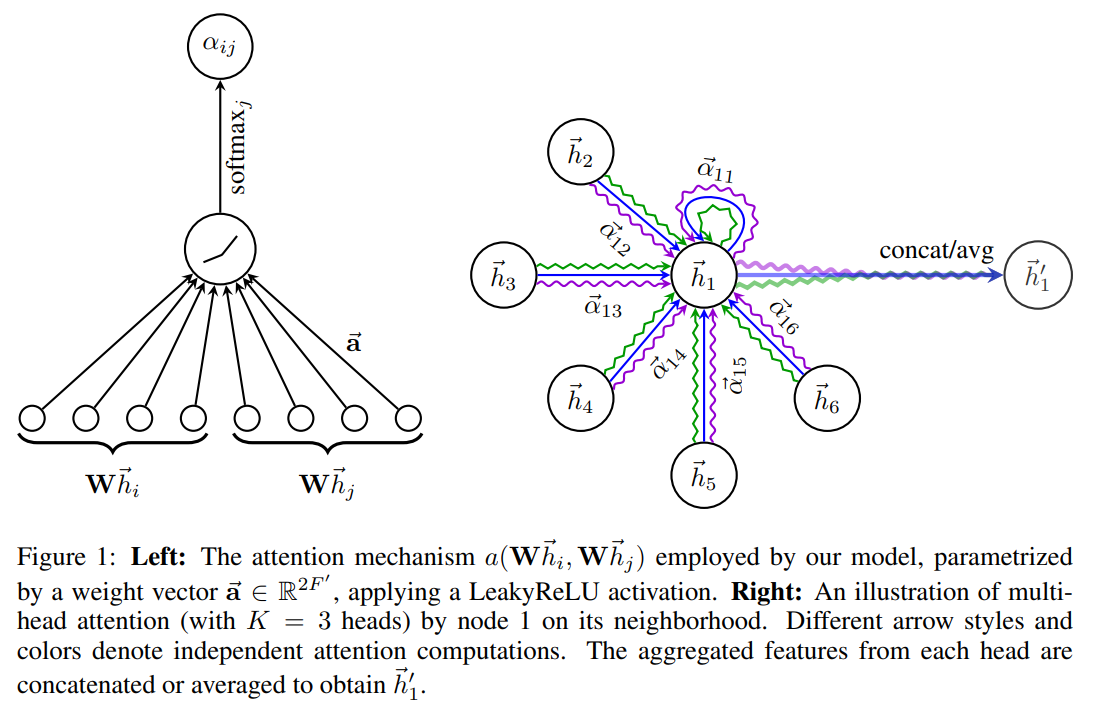
Solution: Learning Attention Weights ($\alpha_{vu}$)
GATs learn attention weights $\alpha_{vu}$ that determine how much each neighbor $u$ contributes to updating the central node $v$.
The GAT update rule at layer $k$ is:
$$\mathbf{h}_v^{(k)} = \sigma\left(\sum_{u \in \mathcal{N}(v)} \alpha_{vu} \cdot \mathbf{W}^{(k)} \mathbf{h}_u^{(k-1)}\right)$$where $u \in \mathcal{N}(v)$ includes the node $v$ itself (self-attention), allowing it to retain its own information while incorporating neighbor features.
Stage 1: Computing the Raw Attention Score ($e_{vu}$)
The score $e_{vu}$ measures the relevance between $v$ and $u$.
$$ e_{vu} = \text{ELU}\left(\mathbf{a}^T [\mathbf{W}\mathbf{h}_v \,||\, \mathbf{W}\mathbf{h}_u \,||\, \mathbf{f}_{vu}]\right) $$where $||$ denotes concatenation (stacking vectors end-to-end).
Breaking down the components:
- Feature Transformation: Both the central node and neighbor features are first transformed using the learned weight matrix $\mathbf{W}$
- Edge Features ($\mathbf{f}_{vu}$): For molecular graphs, these encode bond properties: bond type (single/double/triple/aromatic), bond length, stereochemistry, and whether the bond is in a ring structure
- Concatenation: The transformed features of the central node ($\mathbf{W}\mathbf{h}_v$), the neighbor ($\mathbf{W}\mathbf{h}_u$), and the edge features ($\mathbf{e}_{vu}$) are stacked together
- The Attention Vector ($\mathbf{a}$): This is a trainable parameter (learned via backpropagation) that acts as a simple neural network layer to compute a scalar score from the concatenated features
- ELU Activation: This is used instead of standard ReLU to allow small negative gradients, preventing attention weights from getting stuck at zero during training
Tracking dimensions: If node features have dimension $d_{in} \times 1$, and $\mathbf{W}$ has dimension $d_{out} \times d_{in}$, then:
- After transformation: $\mathbf{W}\mathbf{h}_v$ and $\mathbf{W}\mathbf{h}_u$ each have dimension $d_{out} \times 1$
- Concatenation creates a vector of dimension $(2d_{out} + d_{edge}) \times 1$
- The attention vector $\mathbf{a}$ has dimension $(2d_{out} + d_{edge}) \times 1$
- Result: $\mathbf{a}^T [\mathbf{W}\mathbf{h}_v \,||\, \mathbf{W}\mathbf{h}_u \,||\, \mathbf{f}_{vu}]$ produces a single scalar $e_{vu}$ (dimension $1 \times 1$) as this is a dot product between two vectors
Stage 2: Normalization (Softmax)
The final attention coefficient $\alpha_{vu}$ is obtained by applying $\text{Softmax}$ to normalize the raw scores across all neighbors:
$$ \alpha_{vu} = \frac{\exp(e_{vu})}{\sum_{u' \in \mathcal{N}(v)} \exp(e_{vu'})} $$This ensures that all attention weights for node $v$ sum to 1, creating a probability distribution over its neighbors.
Multi-Head Attention
To achieve robustness and capture diverse patterns, GAT employs multi-head attention. Each head $i$ has its own independent weight matrix $\mathbf{W}^{(i)}$ and attention vector $\mathbf{a}^{(i)}$ to learn different aspects of neighbor importance.
The outputs from $K$ attention heads are combined either by:
Concatenation (typically used in intermediate layers):
$$\mathbf{h}_v^{(k)} = \mathop{\Vert}_{i=1}^{K} \sigma\left(\sum_{u \in \mathcal{N}(v)} \alpha_{vu}^{(i)} \cdot \mathbf{W}^{(i)} \mathbf{h}_u^{(k-1)}\right)$$Averaging (typically used in the final layer):
$$\mathbf{h}_v^{(k)} = \sigma\left(\frac{1}{K}\sum_{i=1}^{K}\sum_{u \in \mathcal{N}(v)} \alpha_{vu}^{(i)} \cdot \mathbf{W}^{(i)} \mathbf{h}_u^{(k-1)}\right)$$where $\Vert$ denotes concatenation across the $K$ heads.
The Nature of GAT Attention
GAT uses a local, additive attention mechanism, which is fundamentally simpler than the global, multiplicative attention (QKV) used in Transformers:
- GAT is Additive: The relevance score is computed by applying a weight vector ($\mathbf{a}$) to the concatenated features. It focuses only on a node’s immediate neighbors (atoms directly bonded in molecular graphs).
- Transformer is Multiplicative (QKV): The score is computed via the dot product (multiplication) of the Query and Key vectors, typically operating on all elements in a sequence or set.
For molecular graphs, this local attention is actually a feature, not a limitation—we want chemistry-aware attention based on actual chemical bonds, not arbitrary long-range interactions between distant atoms.
Despite the simpler calculation mechanism, both models use multi-head attention to enhance the model’s capacity to learn diverse patterns of neighbor importance.
Interpretability for Drug Discovery
After training, the learned attention weights $\alpha_{vu}$ provide valuable insights into molecular structure-activity relationships. Examining these weights reveals which bonds the model considers most important for predicting a property.
In drug discovery, high-attention bonds often correspond to known pharmacophores—functional groups critical for biological activity. For example:
- Hydrogen bond donors/acceptors may receive high attention for binding affinity prediction
- Aromatic rings may be weighted heavily for membrane permeability
- Charged groups may dominate attention in models predicting protein-ligand interactions
This interpretability allows chemists to understand why a model makes certain predictions, bridging the gap between black-box machine learning and traditional medicinal chemistry knowledge.
Implementation:
from torch_geometric.nn import GATv2Conv
import torch.nn.functional as F
import torch
from torch_geometric.nn import global_mean_pool, global_add_pool


class MoleculeGATv2(torch.nn.Module):
    """
    Graph Attention Network for molecular property prediction using GATv2Conv.

    GATv2Conv offers improved expressiveness and better handling of edge features
    compared to the original GATv2Conv.
    """
    def __init__(
        self,
        num_node_features,
        num_edge_features, # Add num_edge_features parameter
        hidden_dim=64,
        num_classes=1,
        num_heads=4,
        dropout=0.2
    ):
        super(MoleculeGATv2, self).__init__()

        # GATv2 layers with multi-head attention
        # First layer: heads concatenated
        self.conv1 = GATv2Conv(
            num_node_features,
            hidden_dim,
            heads=num_heads,
            concat=True,
            dropout=dropout,
            edge_dim=num_edge_features # Specify edge_dim for edge features
        )

        # Second layer: heads concatenated
        self.conv2 = GATv2Conv(
            hidden_dim * num_heads,  # Input is concatenated heads
            hidden_dim,
            heads=num_heads,
            concat=True,
            dropout=dropout,
            edge_dim=num_edge_features # Specify edge_dim
        )

        # Third layer: heads averaged (not concatenated)
        self.conv3 = GATv2Conv(
            hidden_dim * num_heads,
            hidden_dim,
            heads=num_heads,
            concat=False,  # Average heads for final layer
            dropout=dropout,
            edge_dim=num_edge_features # Specify edge_dim
        )

        # Batch normalization
        self.bn1 = torch.nn.BatchNorm1d(hidden_dim * num_heads)
        self.bn2 = torch.nn.BatchNorm1d(hidden_dim * num_heads)
        self.bn3 = torch.nn.BatchNorm1d(hidden_dim)

        # MLP head
        self.fc1 = torch.nn.Linear(hidden_dim, hidden_dim // 2)
        self.fc2 = torch.nn.Linear(hidden_dim // 2, num_classes)

        self.dropout = dropout

    def forward(self, data):
        x, edge_index, edge_attr, batch = data.x, data.edge_index, data.edge_attr, data.batch

        # GATv2 layer 1, passing edge_attr
        x = self.conv1(x, edge_index, edge_attr=edge_attr)
        x = self.bn1(x)
        x = F.elu(x)  # ELU works well with attention

        # GATv2 layer 2, passing edge_attr
        x = self.conv2(x, edge_index, edge_attr=edge_attr)
        x = self.bn2(x)
        x = F.elu(x)

        # GATv2 layer 3, passing edge_attr
        x = self.conv3(x, edge_index, edge_attr=edge_attr)
        x = self.bn3(x)
        x = F.elu(x)

        # Global pooling
        x = global_mean_pool(x, batch)

        # MLP prediction
        x = self.fc1(x)
        x = F.elu(x)
        x = F.dropout(x, p=self.dropout, training=self.training)
        x = self.fc2(x)

        return x

# Initialize model
model = MoleculeGATv2(
    num_node_features=36,
    num_edge_features=10, # Pass num_edge_features
    hidden_dim=64,
    num_classes=1,
    num_heads=4,
    dropout=0.2
)

print(f"Total parameters: {sum(p.numel() for p in model.parameters())}")


# Extracting Attention Weights (for interpretability):

def get_attention_weights(model, data):
    """
    Extract attention weights from the first GAT layer.
    Shows which atoms the model focuses on.
    """
    model.eval()

    # Forward pass through first layer with return_attention_weights
    x, edge_index, edge_attr = data.x, data.edge_index, data.edge_attr # Include edge_attr
    # Get attention weights from first layer
    _, (edge_index, attention_weights) = model.conv1(
        x, edge_index, edge_attr=edge_attr, return_attention_weights=True # Pass edge_attr
    )

    return edge_index, attention_weights

# Example usage
data = mol_to_graph("CC(=O)O")  # Acetic acid
edge_index, attn = get_attention_weights(model, data)

print("Attention weights for first 5 edges:")
for i in range(min(5, edge_index.shape[1])):
    src, dst = edge_index[:, i]
    weights = attn[i]  # Shape: [num_heads]
    print(f"Edge {src.item()} -> {dst.item()}: {weights.detach().cpu().numpy()}")


# prediction
pred = model(data)
print(f"Predicted logit: {pred.item():.4f}")
Total parameters: 294401
Attention weights for first 5 edges:
Edge 0 -> 1: [0.19470206 0.21984781 0.27020392 0.2467302 ]
Edge 1 -> 0: [0.5418553  0.5482287  0.519141   0.50098497]
Edge 1 -> 2: [0.4868451  0.48873252 0.5155894  0.4423833 ]
Edge 2 -> 1: [0.27872428 0.26841444 0.23641402 0.2993698 ]
Edge 1 -> 3: [0.50171024 0.51037735 0.5290461  0.47196847]
Predicted logit: 0.0170
3.4 Message Passing Neural Networks (MPNN)
The Message Passing Neural Network (MPNN) is a general framework that describes how many $\text{GNNs}$ work, providing a unified view of the process. While $\text{GCN}$ and $\text{GAT}$ can optionally incorporate edge features, $\text{MPNN}$ makes the edge-conditioned message passing explicit and central to its design.
The MPNN Framework
The framework consists of two phases, representing one iteration of a typical $\text{GNN}$ layer:
Phase 1: Message Passing (T iterations)
In this phase, information is exchanged and updated locally between connected nodes.
Message Function ($\text{MSG}$): A message $m_{u \rightarrow v}$ is generated for every bond based on the features of the sender node $u$, the receiver node $v$, and the edge feature $\mathbf{f}_{uv}$.
$$ m_{u \rightarrow v}^{(k)} = \text{MSG}(\mathbf{h}_v^{(k-1)}, \mathbf{h}_u^{(k-1)}, \mathbf{f}_{uv}) $$Aggregation: All incoming messages are combined into a single vector $\mathbf{m}_v$ for the receiver node $v$.
$$ \mathbf{m}_v^{(k)} = \sum_{u \in \mathcal{N}(v)} m_{u \rightarrow v}^{(k)} $$Update Function ($\text{UPDATE}$): The node’s features are updated using its previous state and the aggregated message.
$$ \mathbf{h}_v^{(k)} = \text{UPDATE}(\mathbf{h}_v^{(k-1)}, \mathbf{m}_v^{(k)}) $$
Note: Both $\text{MSG}$ and $\text{UPDATE}$ are typically implemented as small Multilayer Perceptrons ($\text{MLPs}$). The crucial distinction here is that the $\text{MSG}$ function is explicitly dependent on the edge feature $\mathbf{f}_{uv}$.
Phase 2: Readout (Global Pooling)
After $T$ message passing steps (where $T$ is the number of $\text{MPNN}$ layers), a readout function aggregates all final node features into a single, comprehensive graph-level representation:
$$ \mathbf{h}_G = \text{READOUT}(\{\mathbf{h}_v^{(T)} | v \in G\}) $$
from torch_geometric.nn import NNConv

class MoleculeMPNN(torch.nn.Module):
    """
    Message Passing Neural Network with explicit edge feature conditioning.

    Edge features (bond type, conjugation, ring membership, etc.) are
    processed by neural networks to generate edge-specific weight matrices
    for message computation.
    """
    def __init__(
        self,
        num_node_features,
        num_edge_features,
        hidden_dim=64,
        num_classes=1,
        dropout=0.2
    ):
        super(MoleculeMPNN, self).__init__()

        # Edge networks: map edge features to weight matrices
        # Each edge network outputs a matrix of size (in_dim × out_dim)
        # that transforms neighbor features based on the bond properties

        self.edge_network1 = torch.nn.Sequential(
            torch.nn.Linear(num_edge_features, hidden_dim),
            torch.nn.ReLU(),
            torch.nn.Linear(hidden_dim, hidden_dim * num_node_features)
        )

        self.edge_network2 = torch.nn.Sequential(
            torch.nn.Linear(num_edge_features, hidden_dim),
            torch.nn.ReLU(),
            torch.nn.Linear(hidden_dim, hidden_dim * hidden_dim)
        )

        self.edge_network3 = torch.nn.Sequential(
            torch.nn.Linear(num_edge_features, hidden_dim),
            torch.nn.ReLU(),
            torch.nn.Linear(hidden_dim, hidden_dim * hidden_dim)
        )

        # MPNN layers with edge-conditioned message passing
        self.conv1 = NNConv(num_node_features, hidden_dim, self.edge_network1)
        self.conv2 = NNConv(hidden_dim, hidden_dim, self.edge_network2)
        self.conv3 = NNConv(hidden_dim, hidden_dim, self.edge_network3)

        # Batch normalization
        self.bn1 = torch.nn.BatchNorm1d(hidden_dim)
        self.bn2 = torch.nn.BatchNorm1d(hidden_dim)
        self.bn3 = torch.nn.BatchNorm1d(hidden_dim)

        # MLP head for graph-level prediction
        self.fc1 = torch.nn.Linear(hidden_dim, hidden_dim // 2)
        self.fc2 = torch.nn.Linear(hidden_dim // 2, num_classes)

        self.dropout = dropout

    def forward(self, data):
        x, edge_index, edge_attr, batch = (
            data.x, data.edge_index, data.edge_attr, data.batch
        )

        # MPNN layer 1: messages computed using bond-specific weights
        x = self.conv1(x, edge_index, edge_attr)
        x = self.bn1(x)
        x = F.relu(x)
        x = F.dropout(x, p=self.dropout, training=self.training)

        # MPNN layer 2
        x = self.conv2(x, edge_index, edge_attr)
        x = self.bn2(x)
        x = F.relu(x)
        x = F.dropout(x, p=self.dropout, training=self.training)

        # MPNN layer 3
        x = self.conv3(x, edge_index, edge_attr)
        x = self.bn3(x)
        x = F.relu(x)

        # Global pooling (readout function)
        x = global_mean_pool(x, batch)

        # MLP prediction head
        x = self.fc1(x)
        x = F.relu(x)
        x = F.dropout(x, p=self.dropout, training=self.training)
        x = self.fc2(x)

        return x

# Initialize model
model = MoleculeMPNN(
    num_node_features=36,
    num_edge_features=10,  # From bond feature extraction
    hidden_dim=64,
    num_classes=1,
    dropout=0.2
)

# Inspect model architecture
print(f"Total parameters: {sum(p.numel() for p in model.parameters()):,}")
print(f"Trainable parameters: {sum(p.numel() for p in model.parameters() if p.requires_grad):,}")

# Break down parameters by component
edge_net_params = sum(p.numel() for net in [model.edge_network1, model.edge_network2, model.edge_network3] for p in net.parameters())
conv_params = sum(p.numel() for conv in [model.conv1, model.conv2, model.conv3] for p in conv.parameters()) - edge_net_params
mlp_params = sum(p.numel() for layer in [model.fc1, model.fc2] for p in layer.parameters())

print(f"\nParameter breakdown:")
print(f"  Edge networks: {edge_net_params:,} ({edge_net_params/sum(p.numel() for p in model.parameters())*100:.1f}%)")
print(f"  Conv layers: {conv_params:,} ({conv_params/sum(p.numel() for p in model.parameters())*100:.1f}%)")
print(f"  MLP head: {mlp_params:,} ({mlp_params/sum(p.numel() for p in model.parameters())*100:.1f}%)")

# Make predictions on sample molecules
model.eval()
molecules = ["CCO", "CC(=O)O", "c1ccccc1"]  # Ethanol, acetic acid, benzene
names = ["Ethanol", "Acetic Acid", "Benzene"]

print(f"\nSample predictions:")
with torch.no_grad():
    for mol_smiles, name in zip(molecules, names):
        data = mol_to_graph(mol_smiles)
        pred = model(data).item()
        print(f"  {name:12s} ({mol_smiles:12s}): {pred:.3f}")
Total parameters: 697,537
Trainable parameters: 697,537

Parameter breakdown:
  Edge networks: 684,352 (98.1%)
  Conv layers: 10,688 (1.5%)
  MLP head: 2,113 (0.3%)

Sample predictions:
  Ethanol      (CCO         ): -0.182
  Acetic Acid  (CC(=O)O     ): -0.165
  Benzene      (c1ccccc1    ): 0.165
Implementation: NNConv (Neural Network Convolution)
NNConv is a highly effective $\text{MPNN}$ variant that achieves strong edge conditioning by having edge features generate edge-specific transformation matrices.
How NNConv Works: Generating Bond-Specific Filters
- Edge Network: For each edge $(u, v)$ with features $\mathbf{f}_{uv}$ (e.g., single or double bond), a small, dedicated $\text{MLP}$ (the edge network) processes $\mathbf{f}_{uv}$ to generate a unique weight matrix: $$\mathbf{W}_{uv} = \text{EdgeNet}(\mathbf{f}_{uv})$$
- Edge-Conditioned Message: This bond-specific matrix $\mathbf{W}_{uv}$ is applied to the neighbor’s feature $\mathbf{h}_u$ to generate the message $m_{u \rightarrow v}$:
$$m_{u \rightarrow v} = \mathbf{W}_{uv} \mathbf{h}_u$$
Intuition: A single bond will generate one $\mathbf{W}$ that down-weights certain features, while a double bond will generate a different $\mathbf{W}$ that up-weights them. The message is transformed based on the bond type.
- Aggregation: All transformed messages are summed to update the receiving node $v$: $$\mathbf{h}_v^{new} = \sigma\left(\sum_{u \in \mathcal{N}(v)} m_{u \rightarrow v}\right)$$
Tracking Dimensions in NNConv (NNConv Layers 2-3)
The complexity of $\text{NNConv}$ is in ensuring the edge network outputs the correct number of values to form the transformation matrix.
- To transform a feature vector from $d_{in}$ to $d_{out}$ (e.g., $64 \to 64$), the required weight matrix $\mathbf{W}_{uv}$ must be $d_{out} \times d_{in}$ ($64 \times 64$).
- The edge network must therefore output $d_{out} \times d_{in} = 64 \times 64 = 4096$ scalar values, which are then reshaped into $\mathbf{W}_{uv}$.
- In the provided code,
edge_network2is designed to produce $4096$ values, reflecting this requirement.
3.5 Architecture Comparison: GCN, GAT, and MPNN
| Architecture | Edge Features Use | Key Mechanism | How Edge Features Are Used | Strengths | Best For |
|---|---|---|---|---|---|
| GCN | Optional (concatenation) | Uniform aggregation ($\mathbf{\hat{A}}$) | Concatenated to node features: $[\mathbf{h}_v, \mathbf{h}_u, \mathbf{f}_{vu}]$; same aggregation for all edge types | Fast, simple, interpretable baseline | Topology-driven tasks; baseline comparisons |
| GAT/GATv2 | Integrated in attention | Learned attention weights ($\alpha_{vu}$) | Modulate attention scores: $e_{vu} = \text{LeakyReLU}(\mathbf{a}^T [\mathbf{W}\mathbf{h}_v, \mathbf{W}\mathbf{h}_u, \mathbf{f}_{vu}])$; different bonds get different attention but same transformation $\mathbf{W}$ | Adaptively weights neighbors; interpretable attention; moderate edge utilization | When neighbor importance varies; interpretability needed |
| MPNN (NNConv) | Generates weight matrices | Edge-conditioned transformations | Generate unique matrices per bond: $\mathbf{W}_{uv} = \text{EdgeNetwork}(\mathbf{f}_{uv})$; single vs. double bonds produce different transformations | Strongest edge differentiation; explicit bond-type modeling | Bond-critical tasks (reactions, stereochemistry, conjugation) |
Key Distinction: GCN concatenates edge features, GAT uses them to weight neighbor importance, MPNN uses them to generate bond-specific transformation matrices.
3.6 Pooling Strategies
After message passing, we have node-level features. For molecule-level predictions, we need global pooling to aggregate these into a single vector.
from torch_geometric.nn import (
    global_mean_pool,
    global_max_pool,
    global_add_pool,
    GlobalAttention,
    Set2Set
)

from torch_geometric.nn.aggr import AttentionalAggregation


# Assume you have a trained MPNN model and some data
model.eval()
data = mol_to_graph("CCO")  # Example molecule

# Forward pass through conv layers to get node embeddings
with torch.no_grad():
    x = data.x
    edge_index = data.edge_index
    edge_attr = data.edge_attr
    batch = data.batch

    # Pass through all conv layers
    x = model.conv1(x, edge_index, edge_attr)
    x = model.bn1(x)
    x = F.relu(x)

    x = model.conv2(x, edge_index, edge_attr)
    x = model.bn2(x)
    x = F.relu(x)

    x = model.conv3(x, edge_index, edge_attr)
    x = model.bn3(x)
    x = F.relu(x)

    # Now x has shape: (num_nodes, hidden_dim) e.g., (5, 64) for a 5-atom molecule
    # batch has shape: (num_nodes,) e.g., tensor([0, 0, 0, 0, 0])

    hidden_dim = 64  # Your model's hidden dimension

    # 1. Mean pooling
    graph_embed_mean = global_mean_pool(x, batch)
    print(f"Mean pool shape: {graph_embed_mean.shape}")  # (1, 64)

    # 2. Sum pooling
    graph_embed_sum = global_add_pool(x, batch)
    print(f"Sum pool shape: {graph_embed_sum.shape}")  # (1, 64)

    # 3. Max pooling
    graph_embed_max = global_max_pool(x, batch)
    print(f"Max pool shape: {graph_embed_max.shape}")  # (1, 64)

    # 4. Attention pooling
    attention_pool = AttentionalAggregation(
        gate_nn=torch.nn.Linear(hidden_dim, 1)
    )
    graph_embed_attn = attention_pool(x, batch)
    print(f"Attention pool shape: {graph_embed_attn.shape}")  # (1, 64)

    # 5. Set2Set pooling
    set2set_pool = Set2Set(hidden_dim, processing_steps=3)
    graph_embed_s2s = set2set_pool(x, batch)
    print(f"Set2Set pool shape: {graph_embed_s2s.shape}")  # (1, 128) - outputs 2×hidden_dim!
Pooling Trade-offs:
- Mean pooling: Simple, stable across graph sizes, standard baseline choice
- Sum pooling: Preserves total information (required for provably expressive architectures like GIN), but output magnitude scales with molecule size
- Max pooling: Captures strongest signals; useful when a single atom/feature dominates (e.g., reactive functional group in toxicity prediction)
- Attention pooling: Learns which atoms are important for the task; interpretable but adds learnable parameters
- Set2Set: Uses iterative LSTM-based refinement; often achieves best performance on benchmarks but computationally expensive and outputs 2×hidden_dim
Practical recommendation: Start with mean pooling for baseline. Try attention pooling if interpretability matters or Set2Set if you need maximum performance and have computational budget.
4. Training GNNs for Property Prediction
Now let’s put everything together and train a model on a real molecular property prediction task.
4.1 Dataset Preparation
We’ll use a simplified toxicity prediction task. In practice, you’d use datasets like:
- Tox21: Toxicity across 12 assays
- BBBP: Blood-brain barrier penetration
- BACE: Binding affinity to BACE enzyme
- ESOL: Aqueous solubility
4.2 Training Loop
A simple pytorch forward and backward pass plus a callback.
from torch_geometric.loader import DataLoader
from sklearn.metrics import roc_auc_score, accuracy_score
import numpy as np
import pandas as pd
from sklearn.model_selection import train_test_split
import torch


# utility functions

# Convert to graph objects
def create_dataset(smiles_list, labels):
    dataset = []
    for smiles, label in zip(smiles_list, labels):
        try:
            data = mol_to_graph(smiles)
            data.y = torch.tensor([label], dtype=torch.float)
            dataset.append(data)
        except Exception as e:
            print(f"Error processing {smiles}: {e}")
    return dataset


def train_epoch(model, loader, optimizer, criterion, device):
    """Train for one epoch."""
    model.train()
    total_loss = 0

    for batch in loader:
        batch = batch.to(device)
        optimizer.zero_grad()

        # Forward pass
        out = model(batch)
        loss = criterion(out, batch.y.unsqueeze(1)) # Fix: Unsqueeze target tensor

        # Backward pass
        loss.backward()
        optimizer.step()

        total_loss += loss.item() * batch.num_graphs

    return total_loss / len(loader.dataset)


def evaluate(model, loader, criterion, device):
    """Evaluate model."""
    model.eval()
    total_loss = 0
    all_preds = []
    all_labels = []

    with torch.no_grad():
        for batch in loader:
            batch = batch.to(device)
            out = model(batch)
            loss = criterion(out, batch.y.unsqueeze(1)) # Fix: Unsqueeze target tensor

            total_loss += loss.item() * batch.num_graphs

            # Collect predictions
            preds = torch.sigmoid(out).cpu().numpy()
            labels = batch.y.cpu().numpy()

            all_preds.extend(preds)
            all_labels.extend(labels)

    avg_loss = total_loss / len(loader.dataset)

    # Compute metrics
    all_preds = np.array(all_preds)
    all_labels = np.array(all_labels)

    auc = roc_auc_score(all_labels, all_preds)
    acc = accuracy_score(all_labels, all_preds > 0.5)

    return avg_loss, auc, acc

# Example dataset (in practice, load from CSV or database)
data_dict = {
    'smiles': [
        'CC(C)Cc1ccc(cc1)C(C)C',  # Ibuprofen - not toxic
        'CN1C=NC2=C1C(=O)N(C(=O)N2C)C',  # Caffeine - not toxic
        'CC(=O)Oc1ccccc1C(=O)O',  # Aspirin - not toxic
        'CCO',  # Ethanol - not toxic (at low doses)
        'c1ccccc1',  # Benzene - toxic
        'C(Cl)(Cl)(Cl)Cl',  # Carbon tetrachloride - toxic
        'c1cc(ccc1N)N',  # p-Phenylenediamine - toxic
        'C1=CC=C(C=C1)O',  # Phenol - toxic
    ],
    'toxic': [0, 0, 0, 0, 1, 1, 1, 1]  # Binary labels
}

# transform to a dataframe
df = pd.DataFrame(data_dict)


# create the dataset
dataset = create_dataset(df['smiles'].tolist(), df['toxic'].tolist())

# Train/test split
train_data, test_data = train_test_split(
    dataset,
    test_size=0.2,
    random_state=42,
    stratify=[d.y.item() for d in dataset]
)

print(f"Training samples: {len(train_data)}")
print(f"Test samples: {len(test_data)}")

# Setup
device = torch.device('cuda' if torch.cuda.is_available() else 'cpu')

# GAT model
model = MoleculeGATv2(
    num_node_features=36,
    num_edge_features=10,
    hidden_dim=64,
    num_classes=1,
    num_heads=4
).to(device)

# or MPNN model
# model = MoleculeMPNN(
#     num_node_features=36,
#     num_edge_features=10,  # From bond feature extraction
#     hidden_dim=64,
#     num_classes=1,
#     dropout=0.2
# ).to(device)

# Data loaders
train_loader = DataLoader(train_data, batch_size=32, shuffle=True)
test_loader = DataLoader(test_data, batch_size=32, shuffle=False)

# Optimizer and loss
optimizer = torch.optim.Adam(model.parameters(), lr=0.001, weight_decay=1e-5)
criterion = torch.nn.BCEWithLogitsLoss()

# Learning rate scheduler
scheduler = torch.optim.lr_scheduler.ReduceLROnPlateau(
    optimizer, mode='min', factor=0.5, patience=2
)

# Training loop
num_epochs = 30
best_auc = 0

for epoch in range(num_epochs):
    print("-" * 20, " epoch: ", epoch)
    # Train
    train_loss = train_epoch(model, train_loader, optimizer, criterion, device)

    # Evaluate
    train_loss, train_auc, train_acc = evaluate(model, train_loader, criterion, device)
    test_loss, test_auc, test_acc = evaluate(model, test_loader, criterion, device)

    # Update learning rate
    scheduler.step(test_loss)

    # Save best model
    if test_auc > best_auc:
        best_auc = test_auc
        # torch.save(model.state_dict(), 'best_model.pt')

    if epoch % 10 == 0:
        print(f"Epoch {epoch:03d} | "
              f"Train Loss: {train_loss:.4f} | Train AUC: {train_auc:.4f} | "
              f"Test Loss: {test_loss:.4f} | Test AUC: {test_auc:.4f}")

print(f"\nBest Test AUC: {best_auc:.4f}")
4.3 Practical Training Tips
1. Dealing with Class Imbalance:
Many molecular datasets are imbalanced (e.g., 95% non-toxic, 5% toxic):
# Compute class weights
pos_weight = (len(dataset) - sum(d.y.item() for d in dataset)) / sum(d.y.item() for d in dataset)
criterion = torch.nn.BCEWithLogitsLoss(pos_weight=torch.tensor([pos_weight]))
2. Data Augmentation:
For molecules, augmentation is tricky (can’t rotate/flip like images). Options:
- Random SMILES enumeration (same molecule, different atom ordering)
- Molecular conformer sampling (different 3D geometries)
def augment_smiles(smiles, n_augment=5):
    """Generate different SMILES for the same molecule."""
    mol = Chem.MolFromSmiles(smiles)
    if mol is None:
        return [smiles]

    augmented = [smiles]
    for _ in range(n_augment):
        new_smiles = Chem.MolToSmiles(mol, doRandom=True)
        augmented.append(new_smiles)
    return augmented
3. Gradient Clipping:
GNNs can suffer from exploding gradients, especially with deep architectures:
# After loss.backward(), before optimizer.step()
torch.nn.utils.clip_grad_norm_(model.parameters(), max_norm=1.0)
optimizer.step()
5. Connections to AlphaFold and the Drug Discovery Pipeline
5.1 Conceptual Parallels: Message Passing and Triangle Updates
There’s a beautiful conceptual connection between GNN message passing and AlphaFold2’s architecture:
GNNs (this blog):
- Operate on molecular graphs (atoms + bonds)
- Message passing enforces chemical consistency: an atom’s properties should be consistent with its bonded neighbors
- Iterative refinement over $k$ layers captures $k$-hop neighborhoods
- After multiple layers, global molecular properties emerge from local interactions
AlphaFold2 (Blog 3):
- Operates on residue-residue graphs (amino acids + spatial proximity)
- Triangle multiplicative updates enforce geometric consistency: if residues $i$ and $j$ are close, and $j$ and $k$ are close, then $i$ and $k$ must satisfy triangle inequality
- Iterative refinement over 48 Evoformer blocks
- After multiple blocks, global 3D structure emerges from local pairwise constraints
The Common Principle: Both architectures recognize that complex global properties (molecular activity, protein structure) emerge from local interactions propagated iteratively. This is a fundamental insight in geometric deep learning.
Attention Mechanisms:
- GATs use multi-head attention to weight neighbor importance
- AlphaFold’s Evoformer uses multi-head attention in MSA rows/columns
- Both learn to focus on the most relevant parts of the structure
5. Applications of GNNs in Drug Discovery
GNNs in the Drug Discovery Pipeline
GNNs accelerate drug development by rapidly evaluating millions of candidates:
| Pipeline Stage | GNN Role | Example Task |
|---|---|---|
| Hit Discovery | Virtual Screening | Predict binding affinity, toxicity, solubility to filter candidates |
| Lead Optimization | Multi-Objective Optimization | Predict ADMET properties to optimize compounds |
| Preclinical Testing | Early Toxicity Screening | Identify toxic compounds before expensive animal testing |
Integrated AI Workflow: AlphaFold (predict protein structure) → GNNs (evaluate candidates) → Molecular Docking (predict binding pose)
Advanced Applications
Beyond property prediction, GNNs enable:
- Protein-Ligand Binding: Predict binding affinity by encoding both molecule and protein structure
- De Novo Generation: Generate novel molecules with desired properties using VAE/GAN architectures
- Retrosynthesis: Predict synthetic routes and reaction outcomes from chemical databases
6. Limitations and Future Directions
Current Limitations
- 2D Structure Only: Standard GNNs ignore 3D geometry (conformation, stereochemistry) crucial for binding affinity
- Over-Smoothing: Deep networks cause distant node features to become indistinguishable
- Data Scarcity: Require thousands of labeled examples, often unavailable for rare properties
Future Directions
- 3D-Aware GNNs: Models like SchNet and DimeNet incorporate atomic coordinates and are SE(3)-equivariant (rotation/translation invariant)
- Pre-trained Foundation Models: Pre-train on massive unlabeled datasets (like ChemBERTa), then fine-tune with limited task-specific data
- Explainability: Tools like GNNExplainer and attention weight visualization make predictions interpretable for medicinal chemists
7. Conclusion
Key Takeaways
- Graphs are the natural representation for molecules they directly encode chemical structure
- Message passing is the core computational pattern: information flows through bonds, updating atom representations iteratively
- Architecture matters: GCN for baselines, GAT for interpretability, MPNN for edge-dependent tasks
- GNNs are state-of-the-art for molecular property prediction, consistently outperforming fingerprints and SMILES-based models
- Connections to AlphaFold: Both GNNs and AlphaFold use iterative local aggregation to capture global properties. Remember, AlphaFold2 uses the Evoformer and Structure modules that rely on attention mechanisms rather than GNN message passing, though both share the principle of iterative local-to-global information aggregation.
Looking Forward: The Complete Drug Discovery Pipeline
We now have powerful tools for both sides of drug discovery:
- Blog 3 (AlphaFold): Predicts protein target structures
- Blog 4 (This post): Predicts and evaluates drug molecule properties
Next, we’ll explore how to design new molecules:
Blog 5 (Next): Generative Models for De Novo Drug Design
Now that we can predict molecular properties with GNNs, how do we generate new molecules optimized for multiple objectives? We’ll explore:
- A short overview of Variational Autoencoders (VAEs) and Generative Adversarial Networks (GANs) for molecules
- Diffusion models for 3D molecule generation and some theory
- Transformer-based generators (MolGPT, ChemFormer)
Blog 6: Molecular Docking
With AlphaFold structures and GNN-designed molecules, we’ll learn to computationally predict where and how these molecules bind to proteins the critical step connecting computational predictions to biological activity.
The Revolution in Computational Drug Discovery
The combination of AlphaFold (protein structures), GNNs (molecular property prediction), generative models (molecule design), and docking (binding prediction) is compressing a 10-year, $2 billion drug discovery process into computational workflows that run in days.
GNNs building on the same principles of iterative geometric reasoning that powered AlphaFold are at the center of this revolution.
References
Landrum, G.: RDKit: Open-source cheminformatics. http://www.rdkit.org ↩︎
Fey, M., & Lenssen, J. E. (2019). Fast graph representation learning with PyTorch Geometric. arXiv preprint arXiv:1903.02428. ↩︎
Gilmer, J., Schoenholz, S. S., Riley, P. F., Vinyals, O., & Dahl, G. E. (2017, July). Neural message passing for quantum chemistry. In International conference on machine learning (pp. 1263-1272). Pmlr. ↩︎
Kipf, T. N. (2016). Semi-supervised classification with graph convolutional networks. arXiv preprint arXiv:1609.02907. ↩︎
Veličković, P., Cucurull, G., Casanova, A., Romero, A., Lio, P., & Bengio, Y. (2017). Graph attention networks. arXiv preprint arXiv:1710.10903. ↩︎