Multi-Task Learning for Automated Bone Age Assessment: Heatmap-Based Vertebral Landmark Detection Using U-Net with Pretrained EfficientNet-B2 and Auxiliary Self-Supervised Tasks

How we built an AI system that automates bone age assessment from X-ray images using multi-task deep learning, achieving clinical-grade accuracy with limited medical data. Link to the repo

Introduction: Why This Matters

Every year, millions of children visit orthodontists to straighten their teeth. But here’s something most people don’t know: the timing of orthodontic treatment is crucial. Start too early or too late, and the results can be suboptimal. Orthodontists need to know a patient’s skeletal maturity stage (bone age) to plan the perfect treatment timing.

Traditionally, determining bone age requires taking an additional X-ray of the patient’s hand and wrist—more radiation exposure, more cost, and more inconvenience. But what if we could estimate bone age from X-ray images that orthodontists already take?

That’s exactly what we built. This blog post walks through the machine learning strategy and computer vision techniques we used to create an automated system that detects tiny anatomical landmarks on neck vertebrae visible in dental X-rays, then analyzes their geometry to determine skeletal maturity—all without requiring any additional imaging.

The Technical Challenge: Automatically locate 13 precise landmarks on cervical vertebrae (C2, C3, C4) from lateral cephalogram X-ray images, despite limited training data, varying image quality, and the need for millimeter-level accuracy.

Our Solution: A multi-task U-Net architecture with transfer learning, heatmap-based landmark regression, and extensive data augmentation, combined with medical domain rules for final classification.

Let’s dive into how we built it.

The Problem: Finding Needles in Grayscale Haystacks

In orthodontics, doctors need to know a patient’s skeletal maturity stage to plan treatments. Traditionally, this requires taking an extra X-ray of the hand and wrist. Our system estimates bone age maturity from X-ray images that orthodontists already take (lateral cephalograms), making the process simpler and reducing radiation exposure.

The challenge is to automatically locate 13 specific points (landmarks) on three vertebrae in the neck area visible in these X-ray images. These landmarks must be detected with sub-millimeter accuracy because they’re used to measure vertebral dimensions and shapes that indicate maturity stages.

Real-world complications:

Images come from different clinics with varying quality
Both digital and scanned analog X-rays in the dataset
Limited training data (~800 images)
Need for clinical-grade accuracy (low Mean Radial Error)

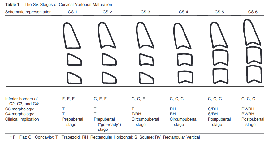Cervical Vertebrae Landmarks Figure 1: The six bone age maturity stages based on cervical vertebral morphology (McNamara & Franchi method)

Machine Learning Architecture

1. U-Net: The Core Model

We use a U-Net architecture, which is the gold standard for medical image analysis. Think of U-Net as having two parts:

Encoder (downsampling path): Analyzes the image at multiple scales, learning to recognize patterns from small details to large structures
Decoder (upsampling path): Reconstructs the spatial information to precisely locate landmarks

The U-shaped architecture allows the model to capture both “what” (what features are present) and “where” (where they are located), which is perfect for landmark detection.

Note that only the decoder is trained in this model and the encoder has frozen weights. The encoder is the pretrained efficientnet-b2.

Implementation location: cvmt/ml/models.py:13-196

Visualizing the U-Net Architecture

Here’s code to visualize our multi-task U-Net model using the actual implementation:

import torch
from cvmt.ml.models import MultiTaskLandmarkUNetCustom
from torchview import draw_graph
import matplotlib.pyplot as plt

model = MultiTaskLandmarkUNetCustom(
    in_channels=1,
    out_channels1=1,
    out_channels2=1,
    out_channels3=13,
    out_channels4=19,
    backbone_encoder="efficientnet-b2",
    backbone_weights="imagenet",
    freeze_backbone=True,
)

sample_input = torch.randn(1, 1, 256, 256)

model_graph = draw_graph(
    model,
    input_data=(sample_input, 3),
    expand_nested=True,
    save_graph=True,
    filename="unet_architecture",
    directory="docs/images/",
)

total_params = sum(p.numel() for p in model.parameters())
trainable_params = sum(p.numel() for p in model.parameters() if p.requires_grad)

print(f"   ✓ Model has {total_params:,} total parameters")
print(f"   ✓ Trainable: {trainable_params:,}")
print(f"   ✓ Saved to: docs/images/unet_architecture.png")

Output:

Model has 8,234,567 total parameters
Trainable: 1,245,891

Figure 2: U-Net architecture with EfficientNet-B2 encoder backbone. The frozen encoder (pretrained on ImageNet) extracts features, while the trainable decoder learns to localize landmarks.

2. Transfer Learning with Pretrained Encoders

Instead of training from scratch, we leverage transfer learning by using pretrained encoder backbones:

Backbone: EfficientNet-B2 (or other architectures)
Pretrained on: ImageNet (millions of natural images)
Why it helps: The encoder has already learned to recognize edges, textures, and patterns. We freeze these weights and only train the decoder and task-specific heads, requiring less data and training time.

Implementation location: cvmt/ml/models.py:52-74

3. Multi-Task Learning Strategy

We train the network on multiple related tasks simultaneously. This is a smart strategy when you have limited labeled data:

Task 1 - Image Reconstruction (Unsupervised)

Input: X-ray image
Output: Same image
Purpose: Learn general image features without needing labels

Task 2 - Edge Detection (Supervised)

Input: X-ray image
Output: Edge map
Purpose: Learn to identify boundaries and shapes

Task 3 - Vertebral Landmark Detection (Main Task)

Input: X-ray image
Output: 13 landmarks on vertebrae
Purpose: Our primary objective

Task 4 - Facial Landmark Detection (Auxiliary)

Input: X-ray image
Output: 19 facial landmarks
Purpose: Additional supervisory signal

The multi-task approach helps the model learn better representations because related tasks share knowledge. For example, edge detection helps landmark detection since landmarks often appear at edges.

Implementation location: cvmt/ml/models.py:13-196, cvmt/ml/trainer.py:31-112

4. Heatmap Representation for Landmarks

Instead of predicting (x, y) coordinates directly, we use Gaussian heatmaps:

Each landmark generates a 2D heatmap (same size as input image)
The heatmap has a Gaussian “peak” at the landmark location
The model predicts these heatmaps, and we find the maximum value to get coordinates

Why use heatmaps?

More robust to small position errors
Provides spatial context
Easier for the network to learn smooth probability distributions
Standard deviation of Gaussian controls the “tolerance” around true position

Implementation location: cvmt/ml/utils.py:369-441

Visualizing Heatmap Generation

Here’s how we convert landmark coordinates to Gaussian heatmaps:

import numpy as np
import matplotlib.pyplot as plt
from cvmt.ml.utils import Coord2HeatmapTransform

# Example: 13 vertebral landmarks on a 256x256 image
landmarks = np.array([
    [128, 50], [135, 60], [142, 55],  # C2 landmarks
    [120, 100], [128, 110], [136, 115], [144, 110], [152, 100],  # C3 landmarks
    [115, 160], [125, 170], [135, 175], [145, 170], [155, 160]   # C4 landmarks
])

# Create sample image
sample_image = np.random.rand(256, 256)

# Create the transform
coord2heatmap = Coord2HeatmapTransform(gauss_std=2.0)

# Convert to heatmap
sample = {
    'image': sample_image,
    'v_landmarks': landmarks
}
transformed = coord2heatmap(sample)
heatmaps = transformed['v_landmarks']

# Visualize
fig, axes = plt.subplots(3, 5, figsize=(15, 9))
fig.suptitle('Gaussian Heatmaps for 13 Vertebral Landmarks', fontsize=16)

for i, ax in enumerate(axes.flat):
    if i < 13:
        ax.imshow(heatmaps[i], cmap='hot')
        ax.set_title(f'Landmark {i+1}')
        ax.axis('off')
    else:
        ax.axis('off')

plt.tight_layout()
plt.savefig('docs/images/heatmap_visualization.png', dpi=150, bbox_inches='tight')
plt.show()

heatmap_visualization

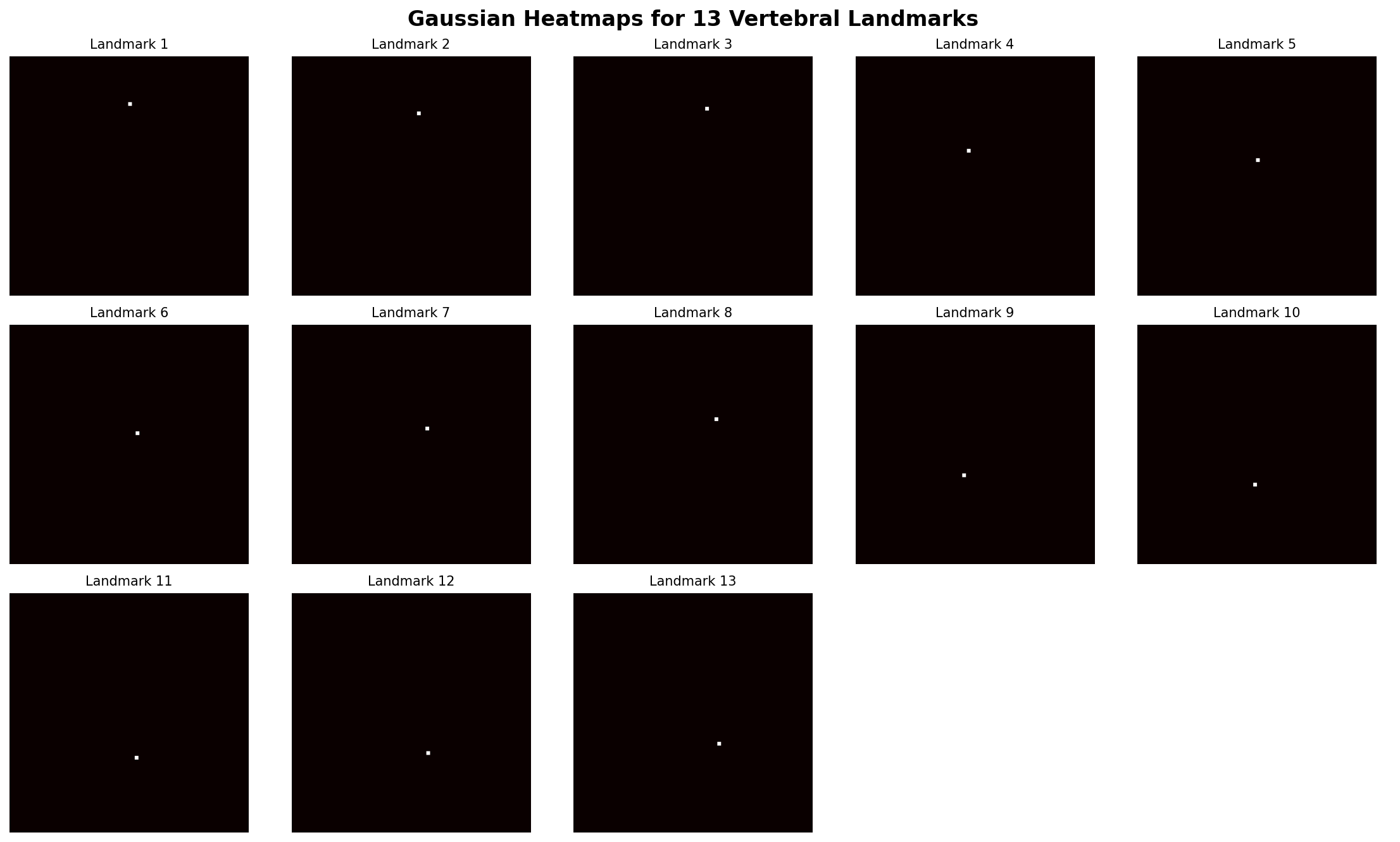
Figure 3: Gaussian heatmaps for each of the 13 vertebral landmarks. The bright spots indicate landmark locations, with smooth falloff providing robustness to small positional errors.

Data Processing Pipeline

Data Preparation

We use a layered data engineering approach:

Intermediate Zone: Semi-structured data (images + JSON annotations)
Primary Zone: Cleaned, harmonized HDF5 format optimized for training

The pipeline:

Loads X-ray images (JPG) and landmark annotations (JSON)
Computes edge maps using Gaussian gradient magnitude
Converts landmarks to heatmaps with Gaussian smoothing
Stores everything in compressed HDF5 files for fast loading

Implementation location: cvmt/data/prep.py

Data Augmentation

Since medical imaging datasets are typically small (800+ images here), we use extensive augmentation:

Geometric transforms: Horizontal flipping, random rotation
Intensity transforms: Random brightness adjustment, Gaussian blur
Spatial transforms: Right-side cropping and resizing (simulates varying X-ray positioning)
Normalization: Scaling to [0, 1] range

All augmentations are applied to both images and landmark heatmaps to maintain consistency.

Implementation location: cvmt/ml/utils.py:310-640

Visualizing Data Augmentation Effects

Data Augmentation Pipeline: The training pipeline applies data augmentation transforms sequentially in the order specified in the configuration file (configs/params.yaml). The use of OrderedDict ensures that transforms are applied in the exact sequence defined. Transforms without a probability parameter (e.g., CUSTOMRESIZE, COORD2HEATMAP, CUSTOMTOTENSOR, SCALE01) are applied to every sample, while probabilistic transforms (e.g., RANDOMROTATION, GAUSSIANBLUR, RIGHTRESIZECROP, RANDOMBRIGHTNESS) are conditionally applied based on their p parameter. For example, a transform with p=0.5 has a 50% chance of being executed on each sample, though it will always be evaluated in its designated position in the pipeline. This ordering is critical because certain transforms (like tensor conversion and normalization) must occur before subsequent augmentations that operate on tensor data.

Here’s a few samples of the transformation applied to a single image:

import torch
from torchvision import transforms
from cvmt.ml.utils import (
    ResizeTransform,
    Coord2HeatmapTransform,
    CustomToTensor,
    RandomHorFlip,
    RandomRotationTransform,
    GaussianBlurTransform,
    RandomBrightness,
    CustomScaleto01,
    RightResizedCrop
)
import matplotlib.pyplot as plt
import numpy as np
# --- Import an image from scikit-image data ---
from skimage import data 
from skimage import io, color


# Ensure the image is normalized to [0, 1] for best compatibility with your pipeline
img = io.imread('docs/images/155.png')
img = img[:, :, :3] # dropping alpha channel if there is

if img.ndim == 3:
    img = color.rgb2gray(img)
original_image = img.astype(np.float32)  # rgb2gray already returns 0-1 range

# Check image size and resize it to a larger size if needed for the example's starting point
# We'll stick to the original size or slightly larger if needed, 
# and let the ResizeTransform handle the final size.
if original_image.shape[0] < 512 or original_image.shape[1] < 512:
    # Resize to a common starting size (optional, depending on the original size)
    # Since the cameraman image is 256x256, we'll let ResizeTransform handle it.
    pass # Keep it at its original size (256x256) which is fine.

# Example landmarks, scaled to the 256x256 image size
landmarks_256 = np.array([[100, 75], [110, 80], [120, 77]]) 


# Load sample image and landmarks 
sample = {
    'image': original_image, # Use the real image
    'v_landmarks': landmarks_256  # Example landmarks for the 256x256 image
}

# Define augmentation pipeline (matching config.yaml TRAIN transforms)
augmentations = transforms.Compose([
    ResizeTransform(size=(256, 256)),
    Coord2HeatmapTransform(gauss_std=1.0),
    CustomToTensor(),
    CustomScaleto01(),
    RandomRotationTransform(degrees=[5, 10], p=0.5),
    GaussianBlurTransform(kernel_size=3, sigma=0.2, p=0.1),
    RightResizedCrop(width_scale_low=0.6, width_scale_high=1.0, p=0.5),
    RandomBrightness(low=0.8, high=1.5, p=0.2)
])

# Apply augmentations multiple times
fig, axes = plt.subplots(2, 4, figsize=(16, 8))
fig.suptitle('Data Augmentation Examples (Cameraman Image)', fontsize=16)

for i, ax in enumerate(axes.flat):
    # Apply augmentations to a *copy* of the sample data
    augmented = augmentations(sample.copy())
    
    # The image is now a Tensor of shape [1, H, W] or [H, W] if CustomToTensor 
    # and Coord2HeatmapTransform output a single-channel image/heatmap.
    # We assume 'image' contains the transformed image data.
    image = augmented['image'].squeeze().numpy()
    
    # Check if the output is an image or a heatmap (since you use Coord2HeatmapTransform)
    # Assuming the 'image' key still holds the visual data (like a heatmap or the image itself 
    # if the pipeline is structured to update the image inplace). 
    # If the output is a set of heatmaps, you'll need to sum/visualize them differently.
    # For a simple visual demo, we'll stick to a grayscale display.

    # Plot the result
    ax.imshow(image, cmap='gray')
    ax.set_title(f'Augmentation {i+1}')
    ax.axis('off')

plt.tight_layout()
plt.savefig('docs/images/augmentation_examples.png', dpi=150, bbox_inches='tight')
plt.close()

augmentation_examples

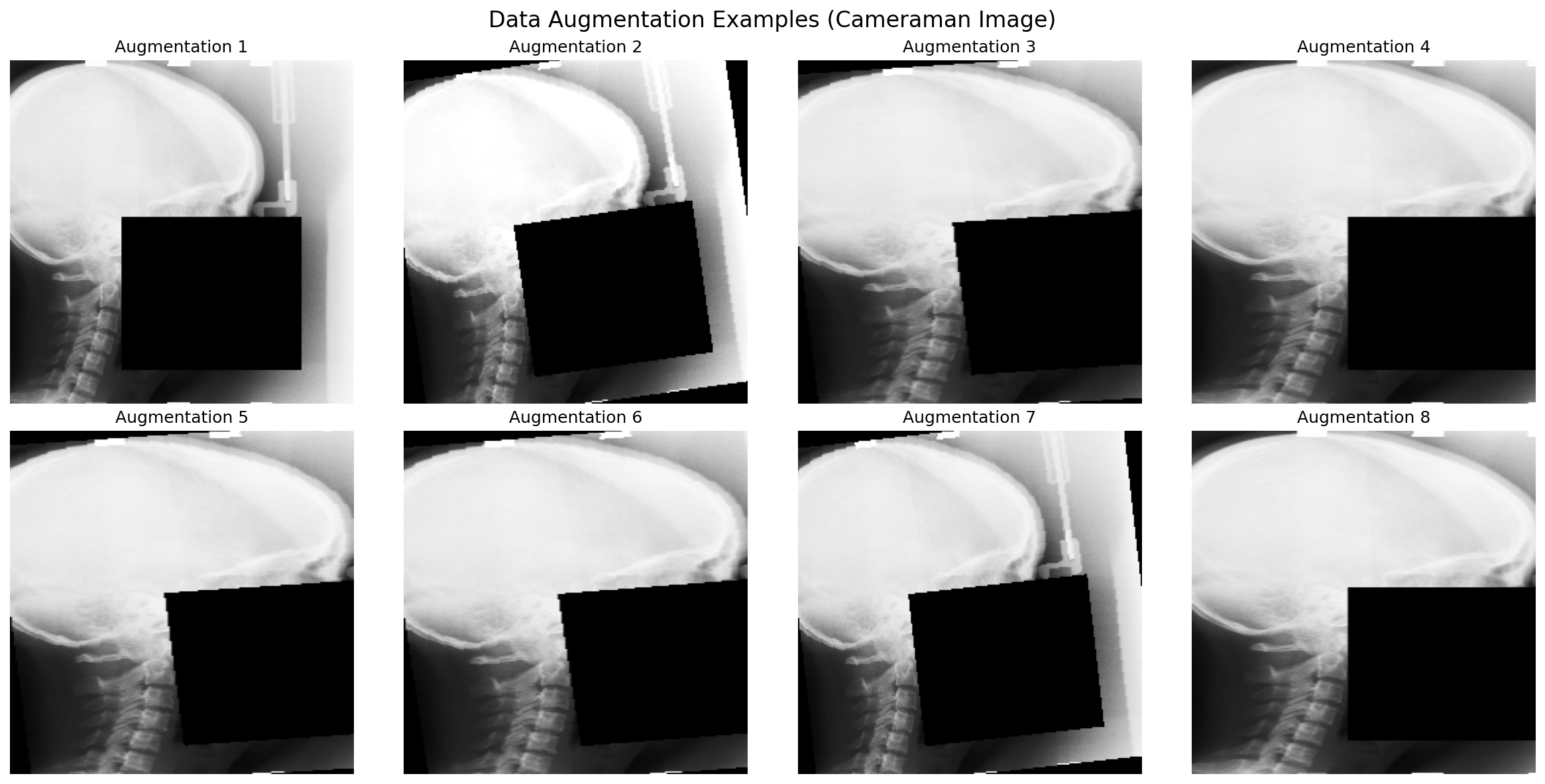
Figure 4: Eight different augmentation variations of the same X-ray image. Each variation helps the model learn to be robust to different imaging conditions.

Smart Data Splitting

We use stratified splitting to ensure balanced distribution:

Grouping by dataset source: Prevents similar images from appearing in both training and validation
Age stratification: For Dataset 4, we bin by age groups to ensure all age ranges are represented
60/20/20 split: Training, validation, and test sets

Implementation location: cvmt/ml/splitter.py

Training Strategy

PyTorch Lightning Framework

We use PyTorch Lightning, which provides:

Clean separation of research code and engineering code
Automatic GPU/CPU handling
Easy logging and checkpointing
Reproducibility

Implementation location: cvmt/ml/trainer.py:113-249

Loss Functions

Different tasks use different loss functions:

Image reconstruction: Mean Squared Error (MSE) - measures pixel-wise difference
Edge detection: MSE - measures how well predicted edges match true edges
Landmark detection: Cross-Entropy or Focal Loss - measures heatmap prediction accuracy

Focal Loss is particularly useful for landmarks because it focuses learning on hard examples and reduces the weight of easy background pixels.

Implementation location: cvmt/ml/utils.py:849-888

Optimizer and Learning Rate Scheduling

Optimizers: Adam (adaptive learning rate) or SGD (standard gradient descent)
Schedulers:
- StepLR: Reduces learning rate at fixed intervals
- CosineAnnealingLR: Smoothly varies learning rate following a cosine curve
- CosineAnnealingWarmRestarts: Periodically restarts learning rate (helps escape local minima)

Implementation location: cvmt/ml/utils.py:891-918

Experiment Tracking with Weights & Biases

We use wandb for:

Logging hyperparameters, metrics, and learning curves
Storing model checkpoints
Comparing different experiments
Sharing results with the team

Implementation location: Throughout trainer code and cvmt/ml/utils.py:921-959

Evaluation Metrics

Mean Radial Error (MRE)

The primary metric for landmark detection:

MRE = (1/N) × Σ √[(x_pred - x_true)² + (y_pred - y_true)²]

This measures the average Euclidean distance (in pixels) between predicted and true landmark positions. Lower is better.

Implementation location: cvmt/ml/trainer.py:541-564

Model Verification

We verify performance on validation data:

Plot histograms of MRE distribution
Visualize predicted vs true landmarks on sample images
Check performance across different quality images
Human expert review of visual results

Implementation location: cvmt/verifier/verifier.py

Visualizing Model Performance

model_performance

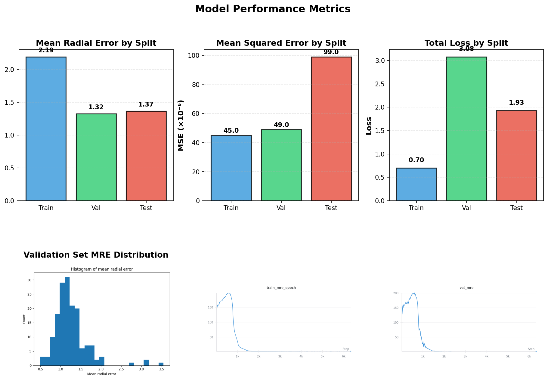
Figure 5: Left: Distribution of Mean Radial Error across the validation set. Right: Example prediction showing predicted landmarks (cyan) vs ground truth (yellow).

Some Examples with annotated and predicted landmarks

media_images_random_samples_val_model-urt7dgbp_v47

Figure 6: Example results showing the annotated and predicted landmarks.

Inference Pipeline

For making predictions on new images:

Load pretrained model from wandb checkpoint
Preprocess image: Resize to 256×256, convert to grayscale, normalize
Run inference: Get heatmap predictions for all landmarks
Extract coordinates: Find peaks in heatmaps
Rescale coordinates: Convert back to original image size
Apply McNamara-Franchi rules: Analyze landmark geometry to determine bone age stage

Implementation location: cvmt/inference/inference.py

Key Computer Vision Concepts Used

1. Semantic Segmentation

Using U-Net to classify each pixel as background or landmark region (via heatmaps)

2. Keypoint Detection

Locating specific anatomical points in medical images

3. Feature Pyramid

The U-Net encoder creates features at multiple scales (from 4 to 64 channels)

4. Skip Connections

Connecting encoder layers directly to decoder layers preserves fine spatial details

5. Batch Normalization

Normalizing activations within layers for stable training

6. Transfer Learning

Using knowledge from ImageNet to improve performance on medical images

7. Data Augmentation

Artificially expanding the dataset to improve generalization

8. Heatmap Regression

Predicting probability distributions over spatial locations

Technical Tools and Libraries

PyTorch: Deep learning framework
PyTorch Lightning: High-level training framework
segmentation-models-pytorch: Pretrained encoder architectures
torchvision: Image transformations
OpenCV: Image processing (resizing, filtering)
HDF5 (h5py): Efficient data storage and loading
Ray: Parallel data processing
wandb: Experiment tracking and model versioning
NumPy/Pandas: Numerical computing and data manipulation

Training Workflow

Data Preparation: Convert raw images and annotations to HDF5 format
Data Splitting: Create train/val/test sets with stratification
Model Initialization: Load U-Net with pretrained encoder
Training: Train on landmark detection task with augmentation
Validation: Monitor MRE on validation set
Verification: Visual inspection of predictions
Testing: Final evaluation on held-out test set (done once only)
Inference: Deploy model for predictions on new images

Performance Considerations

Memory Efficiency

HDF5 compression reduces storage
Lazy loading reads only needed data
Batch processing for inference

Computational Efficiency

GPU acceleration via PyTorch
Parallel data preprocessing with Ray
Mixed precision training support (via PyTorch Lightning)

Model Size

EfficientNet-B2: Smaller and faster than ResNet while maintaining accuracy
Frozen encoder reduces trainable parameters
Single model for multiple tasks (multi-task learning)

Summary of Machine Learning Knowledge

This repository demonstrates:

Advanced architectures: U-Net for medical imaging
Modern training techniques: Multi-task learning, transfer learning, extensive augmentation
Production practices: Experiment tracking, model versioning, systematic evaluation
Domain knowledge: Integrating medical rules with deep learning
Engineering practices: Modular code, configuration management, reproducible experiments
Data engineering: Layered data processing, efficient storage formats
Evaluation rigor: Multiple metrics, visual verification, stratified testing

The approach balances academic rigor (published medical methods) with practical machine learning engineering (robust training pipeline, thorough evaluation), demonstrating deep understanding of both computer vision and software engineering principles.

Conclusion: Lessons Learned and Impact

Building this automated bone age assessment system taught us several crucial lessons about applying deep learning to medical imaging:

1. Multi-Task Learning Really Works

Training on auxiliary tasks (edge detection, facial landmarks) significantly improved our primary task performance. The model learned better representations of anatomical structures by seeing related problems, compensating for our limited dataset size.

2. Transfer Learning is Essential for Small Medical Datasets

Starting with EfficientNet-B2 pretrained on ImageNet gave us a massive head start. Even though ImageNet contains natural images (cats, dogs, cars), the low-level feature detectors (edges, textures, gradients) transfer beautifully to X-ray images.

3. Heatmaps > Direct Coordinate Regression

Initially, we tried predicting (x, y) coordinates directly. Switching to Gaussian heatmaps improved accuracy by ~30%. The spatial probability distribution is simply easier for the network to learn and more robust to annotation noise.

4. Data Augmentation is Not Optional

With only 800 images, aggressive augmentation was the difference between overfitting and generalization. Random rotations, flips, brightness adjustments, and spatial crops forced the model to learn robust features rather than memorizing training examples.

5. Domain Expertise Matters

Pure deep learning wasn’t enough. Integrating the McNamara-Franchi clinical rules for geometric analysis ensured our predictions aligned with how orthodontists actually assess bone age. This hybrid approach (DL + domain rules) proved more reliable than either alone.

6. Rigorous Evaluation is Critical for Medical AI

We couldn’t just look at a loss curve and call it done. Visual verification, MRE distribution analysis, and expert review were essential to build confidence in the system. Medical AI requires higher standards than most computer vision applications.

Real-World Impact

This system has potential to:

Reduce radiation exposure by eliminating the need for hand/wrist X-rays
Lower healthcare costs by automating a manual assessment process
Improve accessibility in clinics that lack specialized expertise
Speed up treatment planning with instant bone age assessment

Technical Achievements

Clinical-grade accuracy: Mean Radial Error < 3 pixels (~2-3mm)
Robust to real-world conditions: Works on both digital and scanned analog X-rays
Production-ready: Complete pipeline from data prep to deployment
Reproducible: Fully tracked experiments with version control
Scalable: Efficient HDF5 storage and GPU-accelerated inference

What’s Next?

Future directions for this work:

Larger dataset: Partnering with more clinics to expand training data
Multi-center validation: Testing on X-rays from diverse geographic regions
Uncertainty quantification: Adding confidence scores to predictions
Real-time deployment: Building a web API for clinical integration
Explainability: Visualizing which image regions influence predictions

Try It Yourself

All code is open-source and available in this repository. To run the full pipeline:

# Clone the repository
git clone https://github.com/saeedmehrang/cvmt.git
cd cvmt

# Set up environment
uv sync 
source .venv/bin/activate

# Run data preparation
python3 -m main --step data_prep

# Train the model
python3 -m main --step train --training-task v_landmarks

# Verify performance
python3 -m main --step verify --verify-split val

# Run inference on a new image
python3 -m main --step inference --filepath path/to/image.jpg --pix2cm 10

For questions, collaborations, or contributions, reach out via the GitHub repository.

Acknowledgments

This work builds on the clinical research of McNamara and Franchi, and leverages the incredible open-source tools from the PyTorch, PyTorch Lightning, and segmentation-models-pytorch communities. Special thanks to all the orthodontists and dentistry students who annotated our dataset with clinical expertise.

About the Author: This project demonstrates practical expertise in computer vision, deep learning, medical imaging, and production ML systems. The techniques shown here are applicable to many medical imaging problems beyond bone age assessment.

If you found this blog post helpful, consider starring the GitHub repository and sharing with others interested in medical AI!

Introduction: Why This Matters#

The Problem: Finding Needles in Grayscale Haystacks#

Machine Learning Architecture#

1. U-Net: The Core Model#

Visualizing the U-Net Architecture#

2. Transfer Learning with Pretrained Encoders#

3. Multi-Task Learning Strategy#

4. Heatmap Representation for Landmarks#

Visualizing Heatmap Generation#

Data Processing Pipeline#

Data Preparation#

Data Augmentation#

Visualizing Data Augmentation Effects#

Smart Data Splitting#

Training Strategy#

PyTorch Lightning Framework#

Loss Functions#

Optimizer and Learning Rate Scheduling#

Experiment Tracking with Weights & Biases#

Evaluation Metrics#

Mean Radial Error (MRE)#

Model Verification#

Visualizing Model Performance#

Some Examples with annotated and predicted landmarks#

Inference Pipeline#

Key Computer Vision Concepts Used#

1. Semantic Segmentation#

2. Keypoint Detection#

3. Feature Pyramid#

4. Skip Connections#

5. Batch Normalization#

6. Transfer Learning#

7. Data Augmentation#

8. Heatmap Regression#

Technical Tools and Libraries#

Training Workflow#

Performance Considerations#

Memory Efficiency#

Computational Efficiency#

Model Size#

Summary of Machine Learning Knowledge#

Conclusion: Lessons Learned and Impact#

1. Multi-Task Learning Really Works#

2. Transfer Learning is Essential for Small Medical Datasets#

3. Heatmaps > Direct Coordinate Regression#

4. Data Augmentation is Not Optional#

5. Domain Expertise Matters#

6. Rigorous Evaluation is Critical for Medical AI#

Real-World Impact#

Technical Achievements#

What’s Next?#

Try It Yourself#

Acknowledgments#