Understanding SwiGLU in Modern Large Language Models

What is SwiGLU?

SwiGLU (Swish-Gated Linear Unit) is an activation function used in the feed-forward networks (FFN) of modern transformer-based language models. It was introduced in the paper “GLU Variants Improve Transformer” by Shazeer (2020) and has since become a standard component in state-of-the-art LLMs like PaLM, LLaMA, and DeepSeek. Follow along to see an interactive visualization where you can see the differences of ReLU, Swish, and SwiGLU on a scalar input x.

Mathematical Definitions

Sigmoid Function

The sigmoid function σ is defined as:

σ(x) = 1 / (1 + e^(-x))

Properties:

Output range: (0, 1)
Smooth, differentiable S-shaped curve
Derivative: σ’(x) = σ(x)(1 - σ(x))

GLU (Gated Linear Unit)

Given an input vector x ∈ ℝ^d and weight matrices W, V ∈ ℝ^(d × d_ff), GLU is defined as:

GLU(x, W, V) = (xW + b) ⊗ σ(xV + c)
                ↑           ↑
              value    sigmoid gate

Where:

⊗ denotes element-wise (Hadamard) multiplication
b, c ∈ ℝ^d_ff are bias vectors
σ is the sigmoid activation function
The sigmoid gate σ(xV + c) controls what information passes through

Swish Function (SiLU)

After GLU demonstrated the power of gating mechanisms, researchers continued searching for better activation functions that could work both standalone and within gated architectures. Swish (also called SiLU) was introduced by Google researchers in 2017 through neural architecture search - essentially, they let AI discover better activation functions automatically. What made Swish special was its self-gating property: unlike GLU which uses a separate sigmoid gate, Swish gates the input with itself (x · σ(x)), creating a smoother, more adaptive non-linearity. This self-gating provides several advantages over simple ReLU or even GLU’s sigmoid: it has continuous derivatives everywhere (no sharp corners like ReLU), it’s unbounded above (preserving large positive values), and crucially, it showed consistent improvements across various deep learning tasks. The success of Swish suggested that combining its smooth, self-gated properties with GLU’s explicit gating mechanism could yield even better results - and this hypothesis led directly to the creation of SwiGLU, which replaces GLU’s simple sigmoid gate with the more sophisticated Swish activation.

The Swish activation function, parameterized by β, is defined as:

Swish_β(x) = x · σ(βx) = x / (1 + e^(-βx))

When β = 1, this is also called SiLU (Sigmoid Linear Unit):

SiLU(x) = x / (1 + e^(-x))

Properties:

Smooth, non-monotonic function
Self-gated: uses its own value for gating
Bounded below by a linear function
As β → ∞, Swish approaches ReLU
Unbounded above: preserves large positive values
Derivative: Swish’(x) = Swish(x) + σ(βx)(1 - Swish(x))

SwiGLU (Swish-Gated Linear Unit)

SwiGLU combines the Swish activation with the GLU gating mechanism, replacing the sigmoid gate with a Swish gate:

SwiGLU(x, W, V) = Swish(xW + b) ⊗ (xV + c)
                      ↑              ↑
                  Swish gate       value

Expanding the Swish component:

SwiGLU(x, W, V) = [(xW + b) ⊗ σ(xW + b)] ⊗ (xV + c)

Where:

x ∈ ℝ^d_model is the input vector
W, V ∈ ℝ^(d_model × d_ff) are learnable weight matrices
b, c ∈ ℝ^d_ff are learnable bias vectors
d_ff is typically (8/3) × d_model for parameter efficiency
The output dimension is ℝ^d_ff

Key Innovation: The Swish gate provides smoother gradients and better performance than the simple sigmoid gate used in GLU.

Complete SwiGLU FFN

In a transformer, the complete SwiGLU feed-forward network includes an output projection:

FFN_SwiGLU(x) = SwiGLU(x, W, V) · W_out + b_out

Where:

W_out ∈ ℝ^(d_ff × d_model) projects back to model dimension
b_out ∈ ℝ^d_model is the output bias
Final output shape matches input: ℝ^d_model

Why Swish Gate Performs Better Than Sigmoid Gate

Theoretical Rationale:

1. Smoother Gradients

Sigmoid: Has very flat gradients when |x| is large (vanishing gradient problem)
Swish: Has non-zero gradients even for negative values, allowing better gradient flow during backpropagation

2. Non-Monotonicity

Sigmoid: Monotonically increasing (always goes up)
Swish: Non-monotonic (has a small “dip” near x ≈ -1.25)
This non-monotonicity allows the network to learn more complex decision boundaries

3. Self-Gating Property

Swish(x) = x · σ(x): The input gates itself
This creates a richer gating mechanism where the magnitude of x influences how much of x passes through
Sigmoid gates don’t have this self-referential property

4. Unbounded Above

Sigmoid: Bounded (0, 1) - compresses all values
Swish: Unbounded above - can preserve large positive values better
This prevents information loss for important features with large magnitudes

Empirical Findings (from Shazeer 2020 paper):

1. Consistent Performance Gains

SwiGLU outperformed GLU variants across multiple tasks
Improvements of 5-8% in perplexity on language modeling benchmarks

2. Better Training Dynamics

Faster convergence during training
More stable training with fewer optimization issues

3. Scalability

Benefits become more pronounced at larger model scales
This is why it’s adopted in billion+ parameter models (LLaMA, PaLM)

Practical Intuition:

Think of it this way:

Sigmoid gate: Binary-ish switch (0 or 1) - “pass or block”
Swish gate: Contextual amplifier - “how much should I amplify this based on its own value?”

The Swish gate can say: “This is a large positive value, let’s keep it large” or “This is slightly negative, let’s attenuate it a bit but not kill it completely” - much more nuanced than sigmoid’s simple on/off behavior.

Interactive Visualization

🧠 Interactive SwiGLU Explorer

Explore how different activation functions behave and understand SwiGLU's gating mechanism

🎛️ Controls

Input Value (x): 0.00

Swish Beta (β): 1.00

Gate Weight (simulated): 1.00

📊 Current Values at x = 0.00

ReLU

0.00

Swish (SiLU)

0.00

SwiGLU Output

0.00

🔬 SwiGLU Formula

SwiGLU(x) = Swish(xW) ⊗ (xV)

where Swish(x) = x · σ(βx)

The ⊗ symbol represents element-wise multiplication (gating). The gate component Swish(xW) controls how much of the linear component (xV) passes through.

The Evolution: From ReLU to SwiGLU

Traditional Feed-Forward Network (ReLU-based)

In early transformers, the feed-forward network used a simple structure:

import numpy as np
import matplotlib.pyplot as plt

# Traditional FFN with ReLU
def relu(x):
    """
    ReLU (Rectified Linear Unit) activation function.
    
    Args:
        x (np.ndarray): Input array of any shape. Each element is processed independently.
    
    Returns:
        np.ndarray: Output array of same shape as input, where each element is max(0, x).
    """
    return np.maximum(0, x)

def traditional_ffn(x, W1, W2, b1, b2):
    """
    Traditional Feed-Forward Network with ReLU activation.
    
    Formula: FFN(x) = ReLU(xW1 + b1)W2 + b2
    
    Args:
        x (np.ndarray): Input tensor of shape (..., d_model) where ... represents 
                        any number of batch/sequence dimensions and d_model is the model dimension.
        W1 (np.ndarray): First weight matrix of shape (d_model, d_ff) where d_ff 
                         is the hidden dimension (typically 4 * d_model).
        W2 (np.ndarray): Second weight matrix of shape (d_ff, d_model) to project 
                         back to model dimension.
        b1 (np.ndarray): First bias vector of shape (d_ff,).
        b2 (np.ndarray): Second bias vector of shape (d_model,).
    
    Returns:
        np.ndarray: Output tensor of shape (..., d_model), same shape as input x.
    """
    hidden = relu(x @ W1 + b1)
    output = hidden @ W2 + b2
    return output

GLU (Gated Linear Unit)

GLU introduced gating mechanisms, splitting the hidden dimension:

def sigmoid(x):
    """
    Sigmoid activation function.
    
    Args:
        x (np.ndarray): Input array of any shape.
    
    Returns:
        np.ndarray: Output array with values in range (0, 1).
    """
    return 1 / (1 + np.exp(-x))

def glu(x, W, V, b, c):
    """
    GLU (Gated Linear Unit) activation function.
    
    Formula: GLU(x) = (xW + b) ⊗ σ(xV + c)
    where ⊗ is element-wise multiplication and σ is the sigmoid function.
    
    Args:
        x (np.ndarray): Input tensor of shape (..., d_model).
        W (np.ndarray): First weight matrix of shape (d_model, d_ff) for the value component.
        V (np.ndarray): Second weight matrix of shape (d_model, d_ff) for the gate component.
        b (np.ndarray): Bias vector for value component of shape (d_ff,).
        c (np.ndarray): Bias vector for gate component of shape (d_ff,).
    
    Returns:
        np.ndarray: Output tensor of shape (..., d_ff) where the value component is 
                    element-wise multiplied by the sigmoid-gated component.
    """
    # Value component (linear transformation)
    value = x @ W + b
    
    # Gate component (sigmoid activation)
    gate = sigmoid(x @ V + c)
    
    # Element-wise multiplication: value gated by sigmoid
    return value * gate

Swish Activation

def swish(x, beta=1):
    """
    Swish activation function (also known as SiLU - Sigmoid Linear Unit when beta=1).
    
    Formula: Swish(x) = x * σ(βx) where σ is the sigmoid function.
    
    Args:
        x (np.ndarray): Input array of any shape. Each element is processed independently.
        beta (float, optional): Scaling parameter for the sigmoid. Default is 1.
                                Higher beta makes Swish behave more like ReLU,
                                lower beta makes it more linear.
    
    Returns:
        np.ndarray: Output array of same shape as input, with Swish activation applied 
                    element-wise.
    """
    return x * sigmoid(beta * x)

SwiGLU: The Modern Standard

SwiGLU combines the Swish activation function with GLU’s gating mechanism:

def swiglu(x, W, V, b, c, beta=1):
    """
    SwiGLU (Swish-Gated Linear Unit) activation function.
    
    Formula: SwiGLU(x) = Swish(xW + b) ⊗ (xV + c)
    where ⊗ is element-wise multiplication.
    
    Args:
        x (np.ndarray): Input tensor of shape (..., d_model).
        W (np.ndarray): First weight matrix of shape (d_model, d_ff) for the gate component.
        V (np.ndarray): Second weight matrix of shape (d_model, d_ff) for the value component.
        b (np.ndarray): Bias vector for gate component of shape (d_ff,).
        c (np.ndarray): Bias vector for value component of shape (d_ff,).
        beta (float, optional): Swish activation parameter. Default is 1.
    
    Returns:
        np.ndarray: Output tensor of shape (..., d_ff) where the Swish-activated gate 
                    component is element-wise multiplied by the linear value component.
    """
    # Gate component (Swish activation) - controls information flow
    gate = swish(x @ W + b, beta)
    
    # Value component (linear transformation) - the actual information
    value = x @ V + c
    
    # Element-wise multiplication: value gated by Swish
    return gate * value

Complete SwiGLU FFN Implementation

Here’s a full implementation of a SwiGLU-based feed-forward network:

class SwiGLU_FFN:
    def __init__(self, d_model, d_ff, beta=1):
        """
        SwiGLU Feed-Forward Network
        
        Args:
            d_model (int): Model dimension (input and output dimension). This is typically
                          the hidden size of the transformer (e.g., 512, 768, 1024, etc.).
            d_ff (int): Hidden dimension for the feed-forward layer. For SwiGLU, this is 
                       typically (8/3) * d_model (approximately 2.67x) to maintain similar 
                       parameter count to traditional FFN with 4 * d_model expansion, while 
                       accounting for SwiGLU's third weight matrix. For example, if d_model=512, 
                       d_ff would be around 1365. See the "Parameter Efficiency" section for 
                       detailed explanation.
            beta (float, optional): Parameter for Swish activation function. Default is 1.
                                   Controls the "sharpness" of the activation.
        """
        self.d_model = d_model
        self.d_ff = d_ff
        self.beta = beta
        
        # Initialize weights (in practice, these would be learned during training)
        # For GLU variants, we need two projection matrices for the gating mechanism
        self.W = np.random.randn(d_model, d_ff) * 0.01      # Gate projection weights
        self.V = np.random.randn(d_model, d_ff) * 0.01      # Value projection weights
        self.W_out = np.random.randn(d_ff, d_model) * 0.01  # Output projection weights
        
        self.b = np.zeros(d_ff)          # Gate projection bias
        self.c = np.zeros(d_ff)          # Value projection bias
        self.b_out = np.zeros(d_model)   # Output projection bias
    
    def forward(self, x):
        """
        Forward pass through SwiGLU FFN
        
        Args:
            x (np.ndarray): Input tensor of shape (batch_size, seq_len, d_model) or 
                           (..., d_model) for any number of leading dimensions.
                           Represents the input embeddings or hidden states.
        
        Returns:
            np.ndarray: Output tensor of shape (batch_size, seq_len, d_model) or 
                       (..., d_model), same shape as input. Represents the transformed
                       hidden states after passing through the SwiGLU FFN.
        """
        # Gate component: Swish(xW + b) - controls what information passes through
        gate_linear = x @ self.W + self.b
        gate = swish(gate_linear, self.beta)  # Apply Swish activation to gate
        
        # Value component: xV + c - the actual information to be gated
        value = x @ self.V + self.c
        
        # Gated output: element-wise multiplication of gate and value
        hidden = gate * value
        
        # Project back to model dimension
        output = hidden @ self.W_out + self.b_out
        
        return output

# Example usage
d_model = 512
d_ff = int(8/3 * d_model)  # ~1365, commonly used ratio for SwiGLU
batch_size = 4
seq_len = 10

# Create random input
x = np.random.randn(batch_size, seq_len, d_model)

# Initialize and run SwiGLU FFN
ffn = SwiGLU_FFN(d_model, d_ff)
output = ffn.forward(x)

print(f"Input shape: {x.shape}")
print(f"Output shape: {output.shape}")
print(f"Number of parameters: {(d_model * d_ff * 2) + (d_ff * d_model)}")

Input shape: (4, 10, 512)
Output shape: (4, 10, 512)
Number of parameters: 2096640

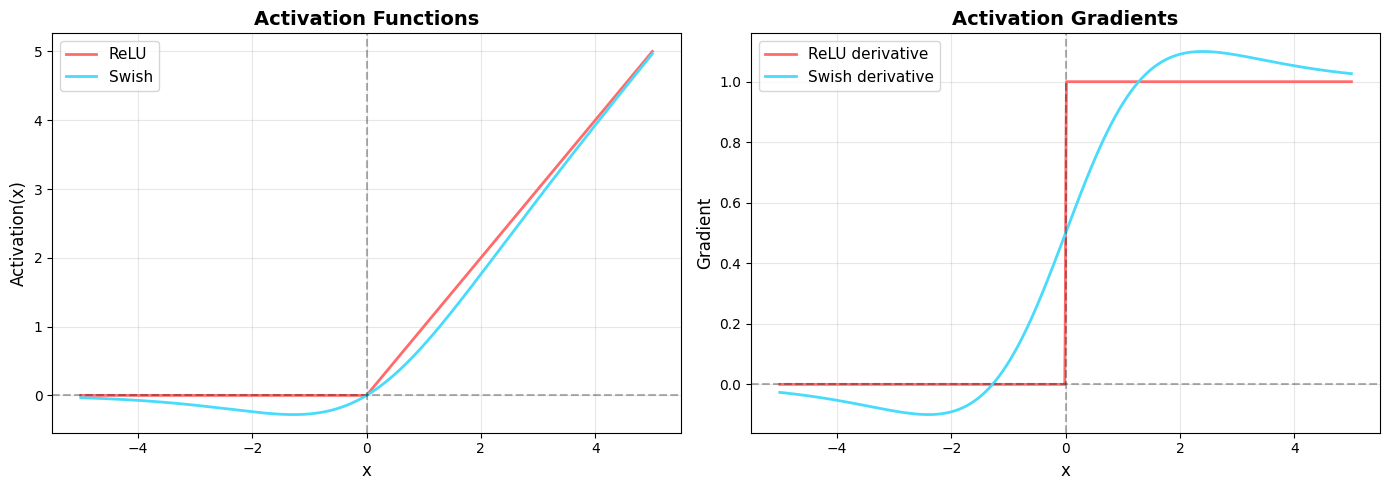
Visualization: Activation Functions and Their Derivatives

# Visualization of activation functions and their derivatives
x = np.linspace(-5, 5, 1000)

# Activations
relu_vals = relu(x)
swish_vals = swish(x)

# Derivatives (computed numerically for visualization)
dx = x[1] - x[0]
relu_grad = np.gradient(relu_vals, dx)
swish_grad = np.gradient(swish_vals, dx)

fig, (ax1, ax2) = plt.subplots(1, 2, figsize=(14, 5))

# Plot activations
ax1.plot(x, relu_vals, label='ReLU', linewidth=2, color='#ff6b6b')
ax1.plot(x, swish_vals, label='Swish', linewidth=2, color='#48dbfb')
ax1.axhline(y=0, color='k', linestyle='--', alpha=0.3)
ax1.axvline(x=0, color='k', linestyle='--', alpha=0.3)
ax1.set_xlabel('x', fontsize=12)
ax1.set_ylabel('Activation(x)', fontsize=12)
ax1.set_title('Activation Functions', fontsize=14, fontweight='bold')
ax1.legend(fontsize=11)
ax1.grid(True, alpha=0.3)

# Plot gradients
ax2.plot(x, relu_grad, label='ReLU derivative', linewidth=2, color='#ff6b6b')
ax2.plot(x, swish_grad, label='Swish derivative', linewidth=2, color='#48dbfb')
ax2.axhline(y=0, color='k', linestyle='--', alpha=0.3)
ax2.axvline(x=0, color='k', linestyle='--', alpha=0.3)
ax2.set_xlabel('x', fontsize=12)
ax2.set_ylabel('Gradient', fontsize=12)
ax2.set_title('Activation Gradients', fontsize=14, fontweight='bold')
ax2.legend(fontsize=11)
ax2.grid(True, alpha=0.3)

plt.tight_layout()
plt.savefig('activation_comparison.png', dpi=300, bbox_inches='tight')
plt.show()

print("Key observations:")
print("- ReLU has a discontinuous gradient at x=0 (sudden jump)")
print("- Swish has smooth, continuous gradients")
print("- Swish allows small negative values to pass through (unlike ReLU)")

Swish vs Relu

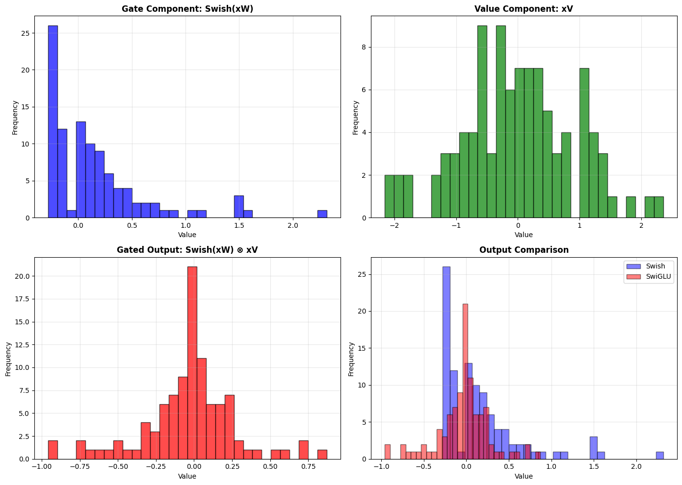
Visualization: Gating Mechanism

# Demonstration of gating effect
np.random.seed(42)
sample_input = np.random.randn(100)

# Create weight matrices for demonstration
W_demo = np.random.randn(100, 100) * 0.1
V_demo = np.random.randn(100, 100) * 0.1

# Without gating (traditional)
swish_output = swish(sample_input @ W_demo)

# With gating (SwiGLU)
gate_part = swish_output                      # GATE: Swish-activated component
linear_part = sample_input @ V_demo           # VALUE: Linear component
swiglu_output = gate_part * linear_part       # GATED OUTPUT

fig, axes = plt.subplots(2, 2, figsize=(14, 10))

# Plot gate component
axes[0, 0].hist(gate_part, bins=30, alpha=0.7, color='blue', edgecolor='black')
axes[0, 0].set_title('Gate Component: Swish(xW)', fontsize=12, fontweight='bold')
axes[0, 0].set_xlabel('Value')
axes[0, 0].set_ylabel('Frequency')
axes[0, 0].grid(True, alpha=0.3)

# Plot linear component
axes[0, 1].hist(linear_part, bins=30, alpha=0.7, color='green', edgecolor='black')
axes[0, 1].set_title('Value Component: xV', fontsize=12, fontweight='bold')
axes[0, 1].set_xlabel('Value')
axes[0, 1].set_ylabel('Frequency')
axes[0, 1].grid(True, alpha=0.3)

# Plot gated output
axes[1, 0].hist(swiglu_output, bins=30, alpha=0.7, color='red', edgecolor='black')
axes[1, 0].set_title('Gated Output: Swish(xW) ⊗ xV', fontsize=12, fontweight='bold')
axes[1, 0].set_xlabel('Value')
axes[1, 0].set_ylabel('Frequency')
axes[1, 0].grid(True, alpha=0.3)

# Plot comparison
axes[1, 1].hist(swish_output, bins=30, alpha=0.5, color='blue', 
                label='Swish', edgecolor='black')
axes[1, 1].hist(swiglu_output, bins=30, alpha=0.5, color='red', 
                label='SwiGLU', edgecolor='black')
axes[1, 1].set_title('Output Comparison', fontsize=12, fontweight='bold')
axes[1, 1].set_xlabel('Value')
axes[1, 1].set_ylabel('Frequency')
axes[1, 1].legend()
axes[1, 1].grid(True, alpha=0.3)

plt.tight_layout()
plt.savefig('gating_mechanism.png', dpi=300, bbox_inches='tight')
plt.show()

print("\nGating allows the network to:")
print("- Modulate information flow based on context")
print("- Learn which features to emphasize or suppress")
print("- Create more expressive representations")

Swiglu vs Swish

Understanding Parameter Efficiency: Why (8/3) × d_model?

A common point of confusion with SwiGLU is the intermediate dimension ratio. Let’s clarify this carefully.

Traditional FFN (ReLU/GELU) - 2 Weight Matrices

A standard feed-forward network has two weight matrices:

# Traditional FFN structure
# W1: d_model × d_ff  (expansion)
# W2: d_ff × d_model  (projection back)
# Total parameters: 2 × d_model × d_ff

# Standard practice: d_ff = 4 × d_model
# Example: if d_model = 512, then d_ff = 2048

Parameter count: 2 × d_model × d_ff = 2 × d_model × (4 × d_model) = 8 × d_model²

SwiGLU FFN - 3 Weight Matrices

SwiGLU, as a GLU variant, requires three weight matrices:

# SwiGLU FFN structure
# W: d_model × d_ff   (gate path)
# V: d_model × d_ff   (value path)
# W_out: d_ff × d_model  (projection back)
# Total parameters: 3 × d_model × d_ff

# If we naively kept d_ff = 4 × d_model:
# Parameters would be: 3 × d_model × (4 × d_model) = 12 × d_model²
# That's 50% MORE parameters than traditional FFN!

The 2/3 Compensation Rule

To keep parameter count similar to traditional FFN, we apply a 2/3 reduction:

New d_ff = (2/3) × Old d_ff

This compensates for having 3 matrices instead of 2:

3 matrices with (2/3) size ≈ 2 matrices with full size
3 × (2/3) = 2

Combining the Rules: The 8/3 Ratio

Modern LLMs (LLaMA, PaLM, Mistral) want to:

Maintain the 4:1 expansion from original Transformers (proven effective)
Use SwiGLU for better performance
Keep similar parameter count for fair comparison

The math:

Target expansion ratio: 4 × d_model
Apply GLU compensation: (2/3) × 4 × d_model = (8/3) × d_model ≈ 2.67 × d_model

Concrete example:

d_model = 512

# Traditional FFN
d_ff_traditional = 4 * d_model = 2048
params_traditional = 2 * 512 * 2048 = 2,097,152 parameters

# SwiGLU FFN
d_ff_swiglu = (8/3) * d_model ≈ 1365
params_swiglu = 3 * 512 * 1365 = 2,097,120 parameters

# Nearly identical parameter counts!

Key Takeaway

The (8/3) ratio is not arbitrary - it’s the result of:

Starting with the proven 4:1 expansion ratio
Applying the 2/3 reduction to account for the third matrix
Ensuring parameter parity with traditional FFNs

This allows fair performance comparisons: any gains from SwiGLU are due to the activation function itself, not from having more parameters.

Architecture Comparison

SwiGLU fits into the transformer architecture as a drop-in replacement for the traditional FFN layer. In modern transformers using SwiGLU:

Transformer Block Structure:

Input Embeddings
Multi-Head Attention
Add & Norm (residual connection + layer normalization)
Feed-Forward Network (SwiGLU) ← This is where SwiGLU replaces ReLU/GELU FFN
Add & Norm
Output to next layer

The key difference is only in step 4, where the FFN activation changes from simple ReLU/GELU to the gated SwiGLU mechanism, providing better gradient flow and expressiveness without changing the overall architecture.

Real-World Impact

SwiGLU is used in many state-of-the-art models:

LLaMA / LLaMA 2 / LLaMA 3: Meta’s open-source language models
PaLM / PaLM 2: Google’s pathways language model
DeepSeek: State-of-the-art reasoning model
Falcon: Technology Innovation Institute’s LLM
Mistral: Mistral AI’s efficient language models

Summary

Why SwiGLU was invented:

Smoother gradients: Swish activation provides better gradient flow than ReLU and sigmoid
Gating mechanism: Allows selective information flow and better feature learning
Empirical superiority: Consistently outperforms ReLU, GELU, and GLU in practice
Parameter efficiency: Achieves better performance with similar or fewer parameters
Scalability: Benefits increase with model size, making it ideal for billion+ parameter models

Key advantages over predecessors:

Aspect	ReLU	GLU (Sigmoid)	SwiGLU
Gradient smoothness	❌ Discontinuous	✅ Smooth	✅ Smooth
Negative values	❌ Blocked	✅ Gated	✅ Swish-gated
Gating mechanism	❌ None	✅ Sigmoid gate	✅ Swish gate
Self-gating	❌ No	❌ No	✅ Yes
Unbounded above	✅ Yes	❌ No	✅ Yes
Number of matrices	2	3	3
Expressiveness	Low	Medium-High	High
Performance gain	Baseline	+3-5%	+5-8%

The innovation of SwiGLU represents the transformer field’s evolution toward more sophisticated activation functions that better capture complex patterns in language data, leading to more capable and efficient language models.

References and Further Reading

Primary Papers

Shazeer, N. (2020). “GLU Variants Improve Transformer.” arXiv preprint arXiv:2002.05202.
- Paper Link
- The original paper introducing SwiGLU and comparing various GLU variants.
Ramachandran, P., Zoph, B., & Le, Q. V. (2017). “Searching for Activation Functions.” arXiv preprint arXiv:1710.05941.
- Paper Link
- Introduces Swish activation function discovered through neural architecture search.
Dauphin, Y. N., Fan, A., Auli, M., & Grangier, D. (2017). “Language Modeling with Gated Convolutional Networks.” International Conference on Machine Learning (ICML).
- Paper Link
- Introduces Gated Linear Units (GLU) for sequence modeling.

Models Using SwiGLU

Touvron, H., et al. (2023). “LLaMA: Open and Efficient Foundation Language Models.” arXiv preprint arXiv:2302.13971.
- Paper Link
- Meta’s LLaMA models use SwiGLU in their feed-forward networks.
Touvron, H., et al. (2023). “Llama 2: Open Foundation and Fine-Tuned Chat Models.” arXiv preprint arXiv:2307.09288.
- Paper Link
- LLaMA 2 continues using SwiGLU architecture.

Understanding SwiGLU in Modern Large Language Models#

What is SwiGLU?#

Mathematical Definitions#

Sigmoid Function#

GLU (Gated Linear Unit)#

Swish Function (SiLU)#

SwiGLU (Swish-Gated Linear Unit)#

Complete SwiGLU FFN#

Why Swish Gate Performs Better Than Sigmoid Gate#

Theoretical Rationale:#

Empirical Findings (from Shazeer 2020 paper):#

Practical Intuition:#

Interactive Visualization#

🧠 Interactive SwiGLU Explorer

🎛️ Controls

📊 Current Values at x = 0.00

ReLU

Swish (SiLU)

SwiGLU Output

🔬 SwiGLU Formula

The Evolution: From ReLU to SwiGLU#

Traditional Feed-Forward Network (ReLU-based)#

GLU (Gated Linear Unit)#

Swish Activation#

SwiGLU: The Modern Standard#

Complete SwiGLU FFN Implementation#

Visualization: Activation Functions and Their Derivatives#

Visualization: Gating Mechanism#

Understanding Parameter Efficiency: Why (8/3) × d_model?#

Traditional FFN (ReLU/GELU) - 2 Weight Matrices#

SwiGLU FFN - 3 Weight Matrices#

The 2/3 Compensation Rule#

Combining the Rules: The 8/3 Ratio#

Key Takeaway#

Architecture Comparison#

Real-World Impact#

Summary#

References and Further Reading#

Primary Papers#

Models Using SwiGLU#

Understanding SwiGLU in Modern Large Language Models

What is SwiGLU?

Mathematical Definitions

Sigmoid Function

GLU (Gated Linear Unit)

Swish Function (SiLU)

SwiGLU (Swish-Gated Linear Unit)

Complete SwiGLU FFN

Why Swish Gate Performs Better Than Sigmoid Gate

Theoretical Rationale:

Empirical Findings (from Shazeer 2020 paper):

Practical Intuition:

Interactive Visualization

The Evolution: From ReLU to SwiGLU

Traditional Feed-Forward Network (ReLU-based)

GLU (Gated Linear Unit)

Swish Activation

SwiGLU: The Modern Standard

Complete SwiGLU FFN Implementation

Visualization: Activation Functions and Their Derivatives

Visualization: Gating Mechanism

Understanding Parameter Efficiency: Why (8/3) × d_model?

Traditional FFN (ReLU/GELU) - 2 Weight Matrices

SwiGLU FFN - 3 Weight Matrices

The 2/3 Compensation Rule

Combining the Rules: The 8/3 Ratio

Key Takeaway

Architecture Comparison

Real-World Impact

Summary

References and Further Reading

Primary Papers

Models Using SwiGLU